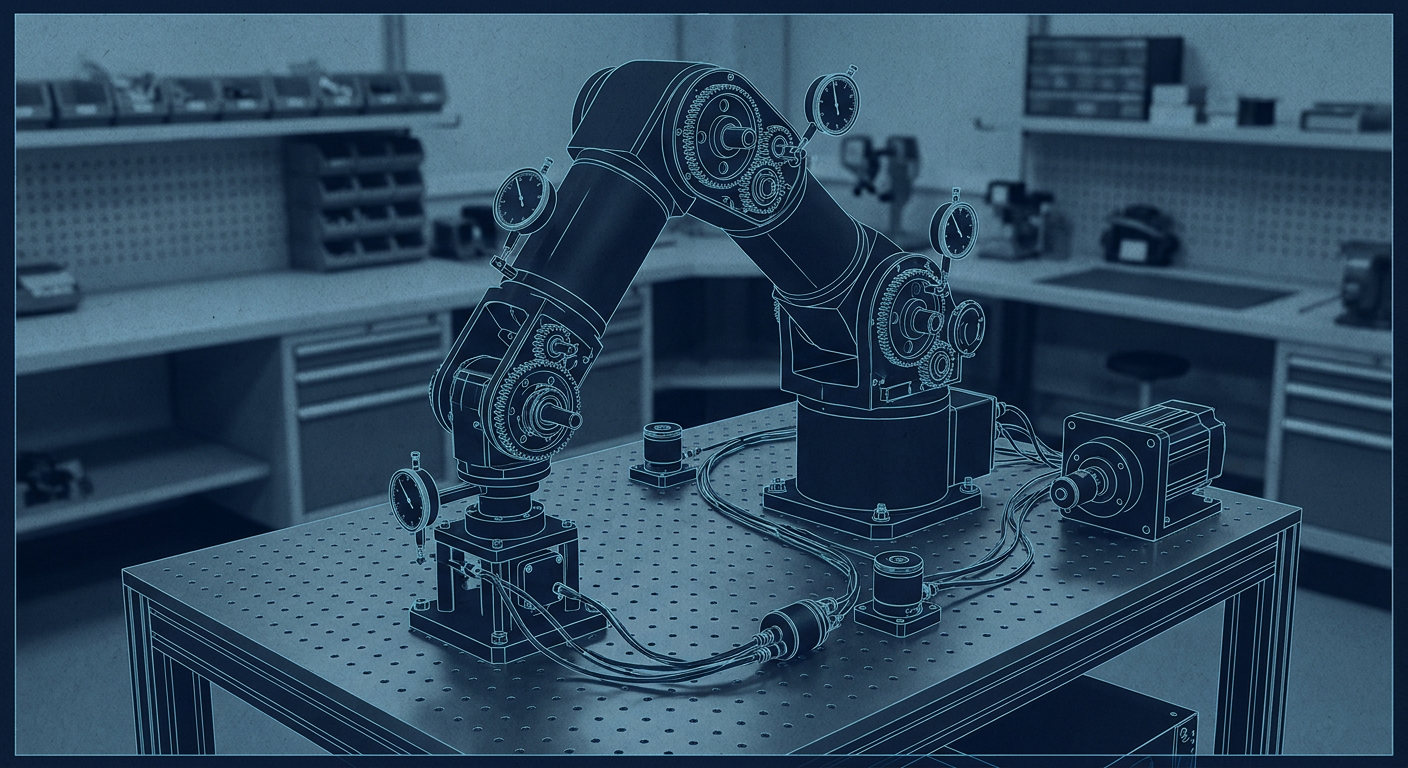
You export a clean URDF from your CAD assembly, bring it into NVIDIA Isaac Sim or MuJoCo, spin up 4,096 parallel environments on an RTX 4090, and watch a reinforcement learning policy converge to millimeter precision in three hours. The simulated robot moves with crisp, damped trajectories. It balances, grasps, and inserts pins into tight-tolerance fixtures without breaking a sweat.
Then you flash the policy to the actual six-axis arm on your workbench.
The physical arm begins to chatter violently at standstill. When it attempts a high-speed trajectory reversal, the end-effector overshoots by four millimeters and rings for 120 milliseconds before settling. After twenty minutes of continuous testing, the arm starts drooping under load because the joint actuators are running at 65 degrees Celsius and their torque-current constant has drifted.
The simulation did not fail because the neural network lacked capacity. It failed because the URDF you exported from your mechanical model is a mathematical fiction. It treats gearboxes as rigid speed reducers, links as infinitely stiff bodies, bearings as frictionless constraints, and motors as ideal torque sources. In the physical shop, none of those assumptions hold.
Closing the reality gap requires treating mechanical non-linearities as first-class physical phenomena inside your simulation pipeline, rather than expecting deep neural networks to magically absorb unmodeled compliance.
The Rigid-Body Assumption in Standard URDF Exports
The standard Unified Robot Description Format (URDF) represents a robot as a kinematic tree of rigid bodies connected by idealized 1-DOF joints. When SolidWorks, PTC Creo, or Fusion 360 outputs a URDF or a USD (Universal Scene Description) file, it calculates the rigid-body mass properties for each link: center of mass, total mass, and the 3x3 inertia tensor around the center of mass.
What it leaves out is everything that happens inside the transmission between the motor shaft and the output flange.
A typical robotic actuator consists of a frameless brushless DC (BLDC) motor, an optical or magnetic rotor encoder, a high-ratio gearbox (typically strain wave or planetary), an output bearing (cross-roller or angular contact), and an output encoder.
When a simulation engine evaluates a revolute joint, it typically calculates the kinematics as:
$$\theta_{link} = \theta_{motor} / N$$
where $N$ is the gear reduction ratio. The joint dynamics are governed by standard rigid-body equations:
$$M(q)\ddot{q} + C(q, \dot{q})\dot{q} + g(q) = \tau$$
On physical hardware, this relationship breaks down. The link position $\theta_{link}$ is decoupled from the motor shaft position $\theta_{motor}$ by three primary non-linearities: transmission compliance, transmission backlash, and friction. If your physics engine assumes the motor rotor is rigidly welded to the joint output link through an ideal ratio $N$, any control policy optimized for fast trajectory tracking will compute feedforward torques that directly excite the structural resonance of the physical gearbox.
Strain Wave Compliance and Non-Linear Torsional Stiffness
Strain wave gears (often referred to by the brand name Harmonic Drive) are standard in collaborative arms and precision industrial robots due to their zero nominal backlash and high single-stage reduction ratios (typically 50:1 to 160:1). They work by using an elliptical wave generator to deflect a thin-walled flexible cup (the flexspline) into progressive engagement with an internal ring gear (the circular spline).
That flexible cup is an intentional torsional spring.
A Harmonic Drive CSF-20-100 gearhead has a non-linear spring characteristic that can be split into three distinct stiffness zones. At low applied torques ($T < T_1$), the flexspline teeth are only lightly seated in the circular spline, yielding a soft torsional spring constant $K_1$. As torque increases toward nominal ratings ($T_1 < T < T_2$), the teeth engage deeper and the stiffness rises to $K_2$. Under peak torques ($T > T_2$), the flexspline walls undergo pure membrane tension, yielding a much stiffer rate $K_3$.
For a standard size 20 unit with a 100:1 ratio, these values look roughly like:
- Low torque zone ($0$ to $7$ Nm): $K_1 \approx 7.5 \times 10^3$ Nm/rad
- Medium torque zone ($7$ to $25$ Nm): $K_2 \approx 1.1 \times 10^4$ Nm/rad
- High torque zone ($> 25$ Nm): $K_3 \approx 1.4 \times 10^4$ Nm/rad
Beyond variable stiffness, strain wave gears exhibit torsional hysteresis. When torque is applied in one direction and then reversed, the load-deflection curve does not retrace its path. The area inside the hysteresis loop represents energy lost to internal material damping and tooth sliding friction. This lost motion (typically 1 to 3 arcminutes) acts like dynamic backlash under low-torque conditions.
When an Isaac Sim policy sends a step command in joint torque, the rigid simulation accelerates the output link instantly. On the bench, the motor rotor turns several degrees before sufficient elastic strain builds up in the flexspline to overcome the static inertia of the downstream link. When the load finally moves, the stored elastic energy releases, inducing a torsional oscillation at the link's natural frequency (typically between 10 Hz and 35 Hz for a loaded 6-axis arm).
If your policy operates at a 50 Hz or 100 Hz control cycle, this resonance lands right inside the controller bandwidth. The policy sees an unexpected phase lag, overcompensates with an opposing torque command, and sends the joint into continuous limit-cycle oscillations.
Planetary Backlash and Deadband Dynamics
While strain wave gears suffer from compliance, planetary gearheads and cycloidal drives suffer from mechanical deadbands.
A precision planetary gearbox (such as an inline Neugart PLE or Apex Dynamics AB series) specified for robotics might guarantee backlash below 3 arcminutes for high-end units, or 10 to 15 arcminutes for standard industrial grades. Lower-cost planetary gearboxes used in budget robotic actuators frequently have 20 to 45 arcminutes of lash.
One arcminute is roughly 0.00029 radians. On a robot arm with a 600 mm reach, 15 arcminutes of backlash at Joint 2 (the shoulder pitch) produces 2.6 mm of free deadband play at the tool center point before any torque is transferred.
In a standard simulation engine, torque transmission is continuous across zero:
$$\tau_{transferred} = \tau_{motor} \cdot N$$
In reality, whenever the torque demand crosses zero (during deceleration or directional reversals), the gear teeth separate. The physical behavior inside the deadband is characterized by three distinct operating regimes:
- Positive Contact: Tooth flank A is engaged. Torque transfer is rigid (plus elastic compliance).
- Free Disengagement: The driven tooth floats across the clearance gap. Transferred torque drops to zero. The motor rotor accelerates freely against its own internal inertia without seeing the link inertia.
- Impact / Re-engagement: Tooth flank B impacts the mating gear. A high-frequency contact force is generated, producing acoustic noise, high instantaneous stress, and a rapid deceleration of the motor rotor.
If an RL policy is trained without deadband modeling, it learns control strategies that rely on infinitesimal torque modulation around zero. When deployed on physical hardware, these small commands leave the gears floating in the backlash zone, resulting in zero link motion followed by violent impact when the policy ramps up torque to overcome the perceived tracking error.
Thermal Drift and Motor Constant Degradation
Simulations assume the actuator's torque constant $K_t$ (Nm/A) and winding resistance $R$ (Ohms) are static parameters. On a real robot working through high-payload pick-and-place cycles, thermal dynamics significantly alter actuator behavior.
The winding resistance of copper wire increases with temperature according to:
$$R(T) = R_0 (1 + \alpha_{Cu} (T - T_0))$$
where $\alpha_{Cu} \approx 0.00393 \text{ K}^{-1}$.
If the stator temperature rises from ambient (25°C) to its continuous operating rating (85°C), the winding resistance increases by roughly 23.6%. Under a bus-voltage-limited regime (such as a 24V or 48V battery-powered mobile manipulator), this resistance increase directly lowers the maximum achievable torque at high joint velocities.
Simultaneously, the remanent magnetic flux density ($B_r$) of the neodymium (NdFeB) permanent magnets on the rotor degrades reversibly with temperature at a rate of roughly -0.11% per degree Celsius. At 85°C, the motor's actual torque constant $K_t$ drops by approximately 6.6%.
$$\tau_{actual} = I_{phase} \cdot K_t(T)$$
A policy relying on open-loop torque estimation or feedforward torque models will apply 6% to 10% less physical torque than it calculated, causing systematic droop and steady-state trajectory errors that worsen over the course of a production shift.
Cable Routing, Energy Chains, and Asymmetric Friction
URDF files rarely include the harness. In real robotic arms, cables for power, Ethernet, CAN-FD, air lines, and sensor feedback must pass through each joint, either externally through corrugated conduit and energy chains, or internally through hollow-shaft actuators.
A heavy cable package routed along a robot arm exerts three physical parasitic forces:
- Position-Dependent Spring Torque: As the joint rotates, the bundled wiring twists or bends, exerting an unmodeled restoring torque that varies with joint angle.
- Hysteresis Friction: The internal rubbing of individual wires against one another and against the outer jacket creates frictional damping that depends on bend radius and temperature.
- Hard Boundary Limits: When an external harness reaches its minimum bend radius, it acts as a stiff, non-linear mechanical stop, resisting motion well before the joint reaches its structural software limit.
Joint friction itself is heavily non-linear. Simulators frequently implement a basic viscous damping coefficient ($c \cdot \dot{q}$). A real actuator exhibits Stribeck friction, which combines static friction (stiction), Coulomb sliding friction, and viscous friction:
$$\tau_f(\dot{q}) = \left( \tau_c + (\tau_s - \tau_c) e^{-|\dot{q}/\dot{q}_s|^{\delta_s}} \right) \text{sgn}(\dot{q}) + b\dot{q}$$
At near-zero velocities, stiction holds the joint stationary until the motor builds sufficient current to break away. Once moving, friction drops before rising again with velocity. If an RL agent does not experience this breakaway drop during training, it will struggle with precision micro-adjustments on the physical bench, repeatedly sticking and then jumping past the target position.
Injecting Mechanical Non-Linearities Back Into Simulation
To bridge the gap between simulation and the shop floor, we must upgrade the mechanical fidelity of our simulation models. You do not need to model every individual gear tooth in finite-element code, but you do need to inject parameterized lumped-element models into the simulation loop.
| Mechanical Non-Linearity | Physical Root Cause | Simulation Failure Mode | Practical Modeling Fix |
|---|---|---|---|
| Flexspline Compliance | Elastic deformation of strain wave cup | High-frequency ringing, phase lag | Series-elastic actuator model with 3-stage stiffness $K(T)$ |
| Gear Backlash | Machining clearance between mating teeth | Impact chatter, loss of low-torque control | Deadband transfer function with restitution coefficient |
| Stribeck Friction | Boundary lubrication in bearings and seals | Stick-slip limit cycles during micro-positioning | Stribeck friction model replacing pure viscous damping |
| Thermal Drift | Magnet heating and copper resistance rise | Systematic joint droop under extended operation | Temperature-dependent $K_t(T)$ derating curves |
| Harness Drag | Elastic bending of routed cables | Angle-dependent trajectory offset | Position-dependent torque bias and friction hysteresis |
1. Two-Mass Series Elastic Modeling
Instead of representing each joint as a single rigid connection between Link $i-1$ and Link $i$, model the actuator as a two-mass system connected by a compliant, damped transmission element.
Split the joint into two states: the rotor position $\theta_m$ (scaled by $N$) and the output link position $\theta_l$. The dynamic torque transmitted across the gearhead is:
$$\tau_{gear} = K_{gear}(\Delta \theta) \cdot (\theta_m/N - \theta_l) + D_{gear}(\Delta \dot{\theta}) \cdot (\dot{\theta}_m/N - \dot{\theta}_l)$$
where $K_{gear}$ is a piece-wise linear function representing the three-zone stiffness curve of your specific gearhead size.
In Isaac Sim or MuJoCo, this can be implemented by inserting an auxiliary dummy link with high rotational inertia (representing the reflected rotor inertia $J_m \cdot N^2$) and defining a custom spring-damper constraint between the dummy link and the actual robot arm link.
2. Explicit Backlash Deadbands
For planetary and cycloidal transmissions, add an explicit deadband operator into the torque calculation:
$$\Delta \theta = \theta_m/N - \theta_l$$
$$\Delta \theta_{engaged} = \begin{cases} \Delta \theta - \beta/2 & \text{if } \Delta \theta > \beta/2 \ 0 & \text{if } |\Delta \theta| \le \beta/2 \ \Delta \theta + \beta/2 & \text{if } \Delta \theta < -\beta/2 \end{cases}$$
where $\beta$ is the measured backlash in radians. Transmitted torque is then calculated using $\Delta \theta_{engaged}$. When the position difference is within the deadband ($|\Delta \theta| \le \beta/2$), transmitted torque is zero, allowing the motor rotor and link masses to accelerate independently.
3. Empirical System Identification on the Bench
Do not rely entirely on catalog numbers for compliance and friction. Gearbox specifications typically provide average values under ideal lubrication and room-temperature conditions. Running a straightforward system identification routine on your assembled hardware will yield accurate lumped parameters.
Set up a test script on your physical arm using the following sequence:
- Locked-Rotor Deflection: Mechanically lock the output flange of Joint $i$ using a rigid steel fixture. Command low-frequency sinusoidal current to the motor ($0.5$ Hz) up to rated torque. Measure motor encoder angle $\theta_m$. Because the output is fixed, $\theta_m/N$ directly maps the non-linear stiffness curve $K(\tau)$ and torsional hysteresis.
- Constant-Velocity Friction Sweep: Unlock the joint and run it across its full range of motion at varying constant velocities, from $0.001 \text{ rad/s}$ up to maximum rated speed. Plot current versus velocity to extract the static friction $\tau_s$, Coulomb friction $\tau_c$, Stribeck velocity threshold $\dot{q}_s$, and viscous damping $b$.
- Harmonic Sweep for Resonance: Command a chirp signal in torque (1 Hz to 100 Hz) at 10% nominal amplitude. Measure the link acceleration with an external IMU or high-resolution secondary encoder on the output side. The resulting Bode plot gives you the exact transmission resonance frequency and structural damping ratio.
Integrating tools like Mexaio AI can help automate the derivation of these dynamic parameters from native CAD geometries, converting raw solid models and assembly tolerances into simulation-ready physical parameters before you even cut metal.
4. Domain Randomization That Reflects Physics
Domain randomization is standard in sim-to-real workflows, but randomizing parameters across arbitrary uniform distributions (such as link mass $\pm 50%$) does not fix fundamental kinematic structure errors. Randomizing link mass will not teach a policy how to handle flexspline hysteresis or backlash crossing.
Instead, structure your domain randomization to target specific mechanical phenomena:
- Gear Stiffness: Randomize $K_1, K_2, K_3$ by $\pm 15%$ around measured values.
- Backlash Gap: Randomize $\beta$ between $0.5 \times \beta_{nominal}$ and $2.0 \times \beta_{nominal}$.
- Stiction and Breakaway Velocity: Randomize $\tau_s$ and $\dot{q}_s$ by $\pm 25%$ to force the policy to learn robust low-speed positioning strategies.
- Transport Delay and Sensor Latency: Add random discrete delays (typically 1 to 4 control steps, representing 10 to 40 ms at 100 Hz) between state observation and actuator command.
- Actuator Thermal Scaling: Randomize the effective motor torque constant $K_t$ between $0.90 \times K_{t,nom}$ and $1.02 \times K_{t,nom}$ to account for coil heating during operation.
Practical Steps for the Shop Floor
Before spending weeks retraining neural networks, take a hard look at your physical prototype and your simulation inputs.
First, check your feedback topology. If your robot arm relies solely on motor-side encoders, the control loop has zero visibility into gear flexure, backlash, or cable pull. Installing high-resolution absolute encoders directly on the link side (after the gearbox) gives your low-level controller the ground-truth link state. A dual-encoder architecture allows you to run high-gain velocity loops on the motor side while closing slow position loops on the link side, mitigating resonance.
Second, inspect your URDF mass matrices. Standard CAD exports often generate unrealistic off-diagonal inertia terms if the origin frames are improperly placed. Zero out negligible off-diagonal terms that fall below the precision threshold of your manufacturing tolerances, and verify that the principal moments of inertia obey the triangle inequalities ($I_{xx} + I_{yy} \ge I_{zz}$).
Third, measure your actual cable harness resistance. Mount an arm horizontally at full extension and record the holding torque required at each joint across its full stroke. If the measured holding torque deviates from the theoretical gravity vector by more than 5%, your cable harness or seal friction is exerting significant unmodeled loads. Add that measured bias curve into your simulation's joint effort limits.
Physical hardware does not obey idealized rigid-body assumptions. When you treat gear compliance, backlash deadbands, thermal limits, and friction dynamics as core simulation parameters rather than rounding errors, policies trained in Isaac Sim will behave on the shop floor exactly as they do on your GPU.
Sources
[1] https://news.mit.edu/2026/ai-agents-create-virtual-playgrounds-to-help-robots-get-crucial-training-data-0713 [2] https://blogs.nvidia.com/blog/icra-research-robotics-simulation-to-real-world/ [4] https://arxiv.org/html/2601.02778v1 [5] https://www.linkedin.com/posts/jerryh01_everyone-in-the-bay-seems-to-be-building-activity-7480008830521745408-hX5o [10] https://docs.nvidia.com/learning/physical-ai/sim-to-real-so-101/latest/03-sim-to-real.html [11] https://aws.amazon.com/blogs/physical-ai/sim-to-real-and-real-to-sim-the-engine-behind-capable-physical-ai/ [13] https://www.worldlabs.ai/blog/real-to-sim-to-real