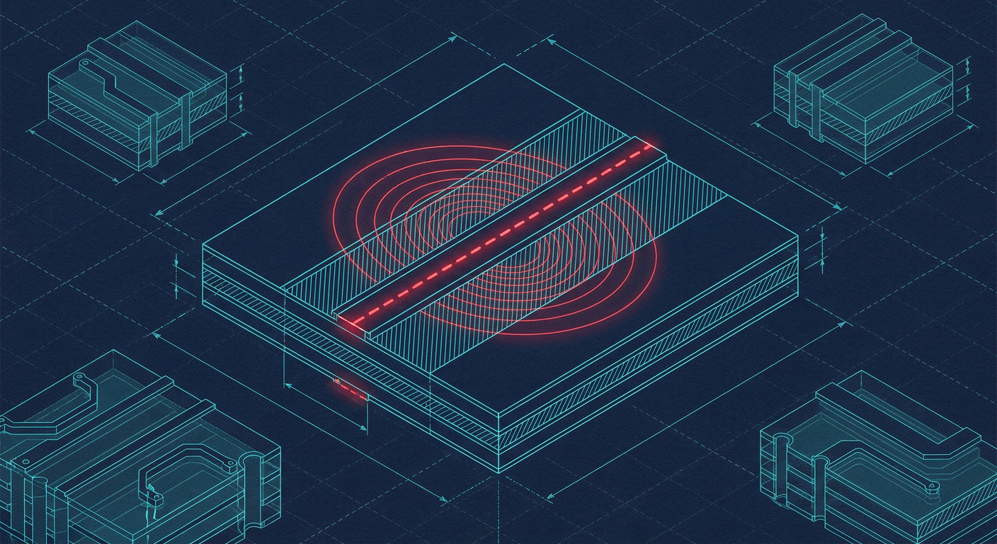
Why AI Autorouters Still Fail at 50-Ohm Controlled Impedance

AI autorouters pass DRC with ease, but they routinely break high-speed return paths. Here is why ML struggles with field physics and how to protect your board.

A four-layer prototype arrives from the fab. The design passed Design Rule Checking (DRC) with zero errors and zero warnings in KiCad or Altium. The traces look tidy, orthogonal, and evenly spaced. But on the bench, the board behaves erratically. The 2.4 GHz RF output from your transceiver is down by 8 dB, the 50-ohm line displays severe ringing on a 500 MHz scope probe, and the prototype fails radiated emissions at 480 MHz during pre-compliance testing.

Every net on that board was fully connected. The clearances met the manufacturer 5-mil trace-and-space rules. The annular rings cleared every pad constraint. Yet the design failed electrically because the autorouter treated copper traces as topological lines on a graph rather than distributed electromagnetic waveguides.

Modern automated routers, whether based on classic Dijkstra and A* pathfinding, Monte Carlo tree search, or reinforcement learning models, solve for geometric connectivity. High-speed signals, however, do not operate on netlist topology. They operate on electromagnetic field boundaries established between a trace and its underlying reference plane. When an automated routing tool does not understand the return path, it creates invisible RF loops, impedance mismatches, and severe signal degradation.

DRC Is a Manufacturing Metric, Not a Physics Engine

A standard PCB design rule check verifies mechanical manufacturability. It checks whether traces are too close to bridge during etching, whether drill holes are too small for plating, and whether soldermask dams are thick enough to prevent solder bridging.

DRC does not calculate capacitance per unit length ($C_0$), loop inductance ($L_0$), or return current distributions. To an automated router operating purely on net connectivity and clearance rules, the three routing topologies below look identical:

A 50-ohm microstrip trace running over an unbroken, solid ground plane.
A 50-ohm microstrip trace crossing a 40-mil gap in a split power/ground plane.
A 50-ohm microstrip trace hopping from Layer 1 to Layer 4 through two vias with no nearby ground return via.

All three options connect Pin A to Pin B with zero short circuits and zero clearance violations. All three pass DRC. But in reality, option 1 delivers a clean step response, option 2 acts as a slot antenna that radiates energy across the chassis, and option 3 creates an inductive discontinuity that can drop the characteristic impedance from 50 ohms down to 35 ohms or spike it past 80 ohms.

Microstrip Cross-Section & Field Distribution

      Trace (Width = W, Thickness = t)
      +-------------------+
      |   Signal Trace    |
      +-------------------+
        | | | | | | | | |    <-- Electric Field Lines (E)
 ~ ~ ~ ~|~|~|~|~|~|~|~|~|~ ~ ~ ~ Dielectric (Height = h, Er)
================================= <-- Continuous Ground Reference Plane
        <--------------->
    Return Current Band (95% within 3h)

The Math of Return Current Distribution

At DC and low frequencies (below a few tens of kilohertz), current takes the path of least resistance. It spreads throughout the copper reference plane in a straight line from the load ground pin back to the power supply ground pin.

At high frequencies (signals with fast rise times, typically anything faster than 1 ns), current takes the path of least inductance. The return current concentrates directly beneath the signal trace on the nearest adjacent reference plane.

For a microstrip line of height $h$ above a reference plane, the return current density $J(x)$ at a lateral distance $x$ from the centerline of the trace follows a distinct distribution:

$$J(x) = \frac{I_0}{\pi h} \frac{1}{1 + (x/h)^2}$$

Where:

$I_0$ is the total signal current.
$h$ is the dielectric height between the signal trace and the reference plane.
$x$ is the lateral distance from the center of the trace.

Over 80 percent of the high-speed return current is contained within a narrow strip of width $3h$ directly under the trace. Over 95 percent is contained within a strip of width $6h$.

If an automated routing algorithm routes that trace over an antipad, a routing slot, or a split between analog and digital planes, the return current cannot travel directly beneath the trace. It must divert around the obstacle.

When the return current diverts, three things happen simultaneously:

Loop Inductance Surges: The loop area between the forward signal and its return path expands. High-frequency loop inductance is directly proportional to loop area. A small 20-mil diversion can add several nanohenries of parasitic series inductance.
Characteristic Impedance Spikes: The characteristic impedance of a transmission line is given by $Z_0 = \sqrt{L/C}$. Increasing the loop inductance without a corresponding increase in capacitance causes $Z_0$ to surge, creating severe impedance discontinuities and signal reflections.
Electromagnetic Radiation Expands: The expanded current loop forms an efficient loop antenna. Radiated electric field strength in the far field scales with loop area and the square of the frequency ($E \propto f^2 \cdot A \cdot I$). A split return path turns a quiet digital signal into an intentional radiator that fails FCC and CE testing.

Broken Return Path Behavior

Signal Layer (Top):  Pin A -----------------------> Pin B
                                      |
Dielectric Gap:                       v
Plane Layer (L2):    [ Solid Ground ] [ Cutout/Split ] [ Solid Ground ]
                                      ^               ^
Return Current Path: <--- Return Path |--- Diverts ---| <--- Return Path
                                     (Loop Area Explodes -> EMI Spikes)

Why AI Routing Models Struggle with Wave Propagation

Many emerging PCB layout tools advertise machine learning or reinforcement learning (RL) backends. While these engines excel at finding legal geometric paths in dense boards, they struggle with high-speed impedance continuity for clear computational reasons.

1. The Computational Cost of Field Solvers

To evaluate the exact characteristic impedance and return path impedance of a trace segment, you must solve Maxwell's equations in two or three dimensions. A 2D boundary element method (BEM) or finite element method (FEM) field solver takes milliseconds to seconds to calculate the impedance and mutual capacitance of a complex cross-section.

An RL routing agent typically takes millions of training steps, evaluating thousands of candidate micro-segments per second. Calling a numerical field solver inside the inner loss loop of an ML model brings the training pipeline to a halt.

To get around this, most AI routers use simplified approximations, such as IPC-2141 formulas or single-layer lookup tables. These formulas assume an ideal, infinite, unbroken reference plane. They calculate that a 12-mil trace on FR4 ($\epsilon_r = 4.2$) with a 6-mil prepreg dielectric equals 50 ohms. The model flags the trace as "50 ohms achieved" regardless of whether that trace is crossing a broken plane, running over a via field, or routing through an adjacent layer cut.

2. The Non-Local Nature of Return Paths

Graph neural networks (GNNs) and convolutional neural networks (CNNs) rely on spatial locality. They evaluate a node or a pixel based on its immediate neighbors.

Return currents are non-local. If a signal hops from Layer 1 to Layer 6 on an 8-layer board, the return current must transition from the Layer 2 ground plane to the Layer 5 ground plane. If there is no ground return via near the signal via, the return current must travel hundreds of mils across the board to find the nearest decoupling capacitor or ground stitch via.

The local geometric patch around the signal via on Layer 1 looks completely valid to the AI model. The failure exists in the global loop physics across the 3D stackup. Capturing this requires full-board 3D electromagnetic modeling, which remains out of reach for real-time iterative routing loops.

Via Layer Transition Discontinuity

Layer 1 (Signal):       Trace IN ======> [ Signal Via ]
Layer 2 (GND Plane):    ==============     | (Cutout)
Layer 3 (Dielectric):                      |
Layer 4 (Dielectric):                      |
Layer 5 (GND Plane):    ==============     | (Cutout)
Layer 6 (Signal):                          +======> Trace OUT

Return Current:         Must find a distant stitch via to jump L2 -> L5.
Displacement current creates high via inductance and impedance dips.

The Four Failure Modes of Automated High-Speed Routing

When automated routing tools operate without rigid boundary constraints, they regularly introduce four specific failure modes.

1. The Broken Reference Plane Split

In mixed-signal or multi-voltage systems, power planes are often split into separate copper islands (such as +3.3V, +1.8V, and +12V). Autorouters frequently route high-speed SPI, I2S, or LVDS traces across the boundaries between these power islands.

Because the plane below changes voltage or ends entirely, the return current is forced to jump the split. The effective capacitance drops, the inductance spikes, and the signal experiences an immediate reflection. At 100 MHz clock speeds, this can introduce 15 to 25 percent edge jitter.

2. Signal Via Transitions Without Ground Stitching

When an automated router encounters dense routing channels, it drops a pair of vias to hop a trace to an internal or bottom layer.

Every signal layer change across a reference plane requires a corresponding return current path. If an autorouter drops four signal vias for a high-speed bus without placing adjacent ground stitching vias within 20 to 30 mils, the return current is blocked. This missing return via introduces between 1.2 nH and 3.5 nH of uncontrolled series loop inductance per transition.

At 6 GHz signal bandwidths (common on USB 3.2 Gen 2 or PCIe Gen 3), this inductance drops the characteristic impedance to 35 ohms or lower, generating a reflection coefficient exceeding -10 dB.

3. Asymmetric Differential Pair Splaying

Differential pairs (such as 90-ohm USB or 100-ohm Ethernet) rely on balanced coupling to reject common-mode noise. Differential impedance is defined as:

$$Z_{diff} = 2 \times Z_{odd}$$

Where $Z_{odd}$ is the impedance of a single trace in the presence of the other driven with opposite polarity.

When an automated router encounters a passive component pad, a connector pinout, or an obstacle, it often splays the positive and negative traces apart to clear DRC. If the spacing $S$ between traces widens while the trace width $W$ remains constant, the odd-mode coupling drops, and the differential impedance jumps immediately from 90 ohms to 115 ohms.

If the router then length-tunes the traces by adding serpentine meanders at the destination connector rather than directly at the point of mismatch, the phase skew creates substantial common-mode voltage, causing the circuit to fail radiated emissions.

Differential Pair Splaying Failure

Balanced (90 Ohm Diff):     Trace+ -------------------
                            Trace- -------------------
                                   <--- Gap S (Tight) --->

Splayed Around Obstacle:    Trace+ -------\       /-------
                                           [ Via ]
                            Trace- -------/       \-------
                                   <--- Gap Spikes -> Z_diff jumps to ~115 Ohm --->

4. Copper Pour Antipad Starvation

In dense multi-layer boards, autorouters cluster vias closely together. The clearance holes (antipads) etched around each via barrel on the inner plane layers overlap.

When three or four antipads merge, they create an accidental slot in the internal ground plane. The router views this as a legal clearance. But to a 50-ohm microstrip running on the surface layer above that via cluster, the ground plane has been completely severed, creating an unreferenced signal segment.

Failure Mode	Root Cause	Impact on SI/EMC	Real-World Symptom
Split Plane Crossing	Trace routes across split power/GND copper	$L_{loop}$ increases, $Z_0$ spikes	Radiated emissions failure at harmonic frequencies
Unstitched Layer Hop	Signal drops via between planes with no GND via	1-3 nH parasitic series inductance	Severe signal ringing, eye diagram closure
Diff Pair Splaying	Asymmetric routing around obstacles	$Z_{diff}$ jumps from 90/100 $\Omega$ to >115 $\Omega$	Packet dropouts, common-mode radiation
Antipad Starvation	Overlapping via cutouts cut plane continuity	Reference plane loss under top traces	Jitter, signal edge degradation

How to Constrain Routing Tools for Clean Signal Integrity

If you use automated routing tools, whether classical EDA autorouters or modern AI-assisted engines like IntelCAD, you cannot hand over the board without strict boundary limits. The tool must be fenced in using electrical and geometric constraints.

1. Build a Symmetrical, Solid-Ground Stackup First

Never use an automated router on a board with an ambiguous stackup. For four-layer boards, use a dedicated ground plane on Layer 2 and a continuous power plane on Layer 3. Do not route random digital control signals on Layer 2.

For six-layer designs, the standard stackup should prioritize reference continuity:

Layer 1: High-Speed Signals / RF (Microstrip over Layer 2 Ground)
Layer 2: Continuous Ground Plane (Zero route cutouts)
Layer 3: High-Speed Signal / Routing (Stripline between Layer 2 and Layer 4)
Layer 4: Continuous Ground Plane or Solid Power Plane
Layer 5: Power / Low-Speed Signals
Layer 6: Low-Speed Signals / Non-critical nets

Ensure that every signal layer is adjacent to at least one continuous, unbroken ground plane.

Recommended 6-Layer Stackup for Automated Routing

L1 (Top):     Signal (RF / High-Speed Controlled Z)   [Microstrip]
----------------------------------------------------- Prepreg (e.g., 4 mil)
L2 (Plane):   GND (100% Solid Reference Plane)
----------------------------------------------------- Core (e.g., 20 mil)
L3 (Signal):  Signal (Stripline High-Speed Routing)
----------------------------------------------------- Prepreg (e.g., 6 mil)
L4 (Plane):   GND / Solid Power Plane
----------------------------------------------------- Core (e.g., 20 mil)
L5 (Signal):  Power Traces / Low-Speed Digital
----------------------------------------------------- Prepreg (e.g., 4 mil)
L6 (Bottom):  Signal / Testpoints / Decoupling

2. Lock and Pre-Route Critical Waveguides Manually

Do not allow an autorouter to touch critical high-speed or RF traces without strict manual supervision. Pre-route the following categories manually and lock them in your EDA tool before running automated engines:

RF Antenna Feeds: 50-ohm single-ended coplanar waveguides with ground stitching.
Switching Nodes (SW): Buck and boost converter switch nodes must remain short, wide, and localized on one layer to prevent inductive spiking ($V = L \frac{di}{dt}$).
Differential Pairs: USB 2.0/3.0, PCIe, HDMI, Ethernet pairs should be routed manually with matched lengths and locked.
Low-Noise Analog Traces: Traces connected to sensitive op-amp inverting inputs or 24-bit ADC inputs.

3. Configure Keep-Out Fences and Antipad Rules

To prevent the router from creating antipad slots in ground planes:

Set minimum via-to-via pitch constraints so that adjacent drill clearances never merge on internal layers. For 0.3 mm drill vias with 0.5 mm pads, keep a center-to-center spacing of at least 0.9 mm to 1.0 mm.
Place explicit routing keep-outs on signal layers directly above any inevitable split in power planes.
Restrict high-speed net classes to specific signal layers (e.g., assign high-speed nets only to Layer 1 and Layer 3) and forbid the router from changing layers on those specific nets.

4. Run Fast Post-Route 2.5D Verification

After the automated router completes its passes, do not send the Gerber files directly to the fab based on a green DRC flag. Run a signal integrity analysis or a manual plane inspection check:

Highlight the Ground Plane: Turn off all signal layers. Examine the ground plane on Layer 2 and Layer 5. Look for Swiss-cheese perforations where dense via clusters have cut off return paths.
Trace the High-Speed Loops: Select each high-speed net and visually follow its path on the adjacent plane layer. If the trace crosses an empty gap in the plane below it, reroute it immediately.
Inspect Differential Via Transitions: Ensure that wherever a differential pair changes layers, a dedicated ground return via is placed within 25 mils of the signal vias.

Clean Ground Via Stitching Pattern

          [ Signal Via + ]    [ Signal Via - ]
                 o                  o

                 O                  O
          [ Ground Via ]      [ Ground Via ]
          (Tied to L2/L5 Ground Planes within 20 mils)

Moving from Geometric Automation to Physics-Aware Routing

Automated routing is moving past basic topological graph searches, but engineers must understand the boundaries of their tools. A router that only tracks coordinates and clearances will always generate boards that pass manufacturing rules while failing electromagnetic compliance.

Until EDA engines incorporate real-time, accelerated 3D boundary-condition verification into their inner optimization loops, you must act as the physics engine. Lock down your stackup, clamp net classes to dedicated reference planes, manually route RF and switching loops, and never trust a clean DRC report until you have verified the return path yourself.