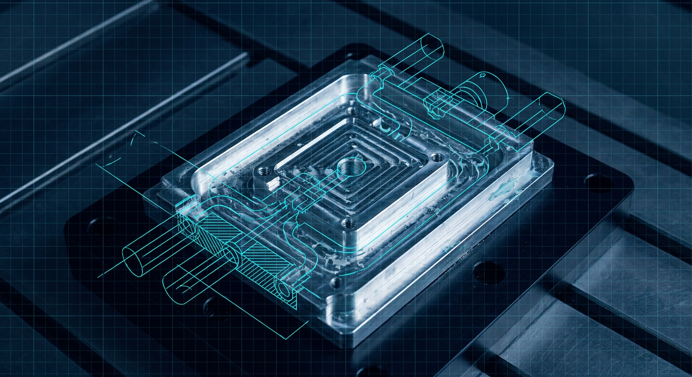
Generative Cold Plates and the Reality of CNC Milling

We benchmarked AI thermal solvers from Diabatix and Neural Concept against Ansys Fluent. Here is what happens when you try to machine the channels.

We spent the last three weeks running a 450W power inverter cold plate through Diabatix ColdStream and Neural Concept Shape, then checking their fluid predictions against our standard Ansys Fluent workflow. The goal was simple. We wanted to see if deep-learning surrogate models and topology optimization algorithms actually shave design cycles off liquid-cooled blocks, or if they just spit out organic geometry that ruins our shop machining budget.

Cooling power electronics is an exercise in compromise. You want to shrink thermal resistance from the IGBT or GaN junction down to the fluid below 0.08 K/W. You also have an onboard miniature gear pump or a restrictive automotive loop that stalls if your cold plate pressure drop climbs past 40 kPa at 4 liters per minute.

Standard engineering practice has relied on serpentine channels, straight fin arrays, or staggered pin-fin matrices. We know how to program a 2mm endmill to cut straight ribs into 6061-T6 aluminum in 18 minutes. We know how to skim the deck flat on a fly cutter to within 0.01mm so the O-ring or vacuum braze foil seals without leaks. The AI tools promise to pull temperatures down by 4°C to 9°C for the exact same pumping power by growing branching, vascular channel trees.

What they do not tell you up front is what happens when those step files hit Mastercam.

The Benchmark Problem and Simulation Setup

To make this test fair, we locked down the boundary conditions on a realistic footprint from an electric actuator drive stage.

Baseplate footprint: 140mm x 90mm x 12mm thickness.
Material: Aluminum 6061-T6 ($k = 167\text{ W/m}\cdot\text{K}$).
Heat source: Four discrete MOSFET heat sources delivering 112.5W each across 15mm x 15mm pads (450W total).
Working fluid: 50/50 Water-Ethylene Glycol (WEG) entering at 40°C.
Inlet flow rate: 3.5 L/min with an upper pressure drop budget of 35 kPa.
Target: Minimize maximum junction surface temperature under the hottest silicon die while keeping manufacturing cost reasonable for a batch run of 250 parts.

In our baseline CAD setup in SolidWorks, we designed two classic architectures. The first was a four-pass serpentine channel with 3mm wide slots and 4mm depth. The second was an offset pin-fin matrix using 1.5mm square pins with 1.5mm spacing across the core heat zone.

Then we set up identical fluid volumes inside Diabatix ColdStream, trained a geometric deep learning model in Neural Concept Shape against historical Navier-Stokes runs, and pushed the baseline models into Ansys Fluent (2024 R1) and SimScale for conjugate heat transfer verification.

+-----------------------+---------------------+-------------------+------------------+
| Architecture          | Max Baseplate Temp  | Pressure Drop     | Solve Time       |
+-----------------------+---------------------+-------------------+------------------+
| Serpentine Baseline   | 68.4°C              | 14.2 kPa          | 42 min (CFD)     |
| Pin-Fin Matrix        | 61.8°C              | 31.8 kPa          | 55 min (CFD)     |
| Neural Concept Model  | 59.2°C              | 28.6 kPa          | 4 seconds (Inf)  |
| Diabatix Generative   | 57.1°C              | 26.4 kPa          | 3.2 hours (Opt)  |
+-----------------------+---------------------+-------------------+------------------+

Where the Solvers Differ: Speed vs Fidelity

Traditional conjugate heat transfer in Ansys Fluent requires a fully resolved fluid boundary layer. To get wall $y^+ \approx 1$ with a standard $k$-$\omega$ SST turbulence model across narrow liquid channels, our meshing pipeline built roughly 6.8 million poly-hexcore cells. Solving momentum, energy, and turbulence equations across that mesh took between 40 and 60 minutes on an 8-core workstation.

If you want to iterate a pin-fin design manually, you change three dimensions in CAD, regenerate the mesh, re-run the solver, and check the delta. An experienced thermal engineer can get through five or six variations a day before running out of patience.

Diabatix approaches this as a density-based topology optimization loop wrapped around an automated finite volume solver running in the cloud. You define the bounding fluid volume, the inlet and outlet ports, the heat flux faces, and the solver iteratively removes fluid resistance and metal volume. It does not just tune parameters. It carves organic bifurcations, thinning channels where thermal gradients are low and expanding surface area right under the heat sources.

The compute time is real. The optimization ran through roughly 220 iterations over 3.2 hours in their cloud environment. But you do not touch it during that window. It outputs an optimized Parasolid or STEP body with fluid channels already mapped.

Neural Concept operates differently. Instead of running a live numerical solver from scratch during the design loop, its PointNet and graph neural network surrogates predict the velocity profiles, surface temperature fields, and pressure drops directly from the 3D surface mesh. Once trained on a family of cold plate geometries, inference takes less than five seconds.

You can drag slider bars or let a rapid genetic algorithm sweep thousands of channel height, taper, and wall thickness permutations in under ten minutes. The output gets you within 3% to 5% of a full Fluent run for global pressure drop and peak temperature, provided your proposed shape stays within the parameter distribution of the training set.

When you step outside the training boundaries, however, surrogate models tend to hide localized flow recirculation zones. In one run, Neural Concept predicted no hot spots on a sharp 90-degree corner divergence, but when we verified the geometry in Fluent, a low-velocity eddy had formed right behind a downstream fin, kicking local baseplate temperature up by 4.2°C higher than the model predicted. You cannot skip final Navier-Stokes verification before cutting metal.

The Machining Floor: Converting Smooth Splines into G-Code

The software output looks incredible on a monitor. The organic fluid channels branch like human capillaries, converging under the GaN dies and dividing smoothly toward the outlet manifold.

Then you export the geometry to your CAM software, and the trouble begins.

Tool Access and Corner Radii

AI generative algorithms love creating variable-width channels with sweeping spline boundaries. If a channel tapers from 3.2mm down to 1.1mm with a curved bottom fillet, you cannot cut that on a 3-axis CNC vertical machining center with standard endmills without continuous tool changes and tiny stepovers.

When we took the unconstrained Diabatix model directly to a Haas VF-2SS:

Minimum internal corner radii dropped to 0.4mm in several transition zones. This demanded a 0.8mm flat endmill running at 12,000 RPM with an extremely conservative feed rate of 180 mm/min to avoid snapping the tool in 6061 aluminum at a 4mm depth of cut.
The total machining time for a single bottom tub plate exploded to 84 minutes. Most of that time was spent rest-milling the micro-radii that the 3mm roughing tool could not reach.
The thin internal walls, generated at 0.6mm thickness by the solver to maximize conduction surface, vibrated under standard tool engagement, creating chatter marks that ruined the channel dimensional tolerances.

If you run topology optimization without strict manufacturing constraints turned on, the software assumes your tool can machine an infinitely sharp internal corner at any arbitrary depth.

To make the generative plate practical for CNC milling, we had to re-run the optimization with hard geometric limits: a minimum feature size of 2.0mm (allowing a 1/16 inch or 1.5mm endmill to clear paths easily), a uniform channel floor depth of 4.5mm, and draft angles compatible with standard cutters.

When we enforced those constraints, the peak thermal performance dropped by about 1.3°C compared to the unconstrained organic shape. However, the machine cycle time on our Haas dropped from 84 minutes down to 22 minutes. That is the difference between a part costing $140 in machine time versus $38 in machine time.

+----------------------------+-------------------+-------------------+------------------+
| Manufacturing Constraint   | Baseplate Max T   | Pressure Drop     | CNC Cycle Time   |
+----------------------------+-------------------+-------------------+------------------+
| Unconstrained Generative   | 57.1°C            | 26.4 kPa          | 84 min           |
| CNC Constrained (2.0mm R)  | 58.4°C            | 27.1 kPa          | 22 min           |
| Standard Milled Serpentine | 68.4°C            | 14.2 kPa          | 18 min           |
+----------------------------+-------------------+-------------------+------------------+

Sealing and Joining: Vacuum Brazing vs O-Rings

A cold plate is not just a milled tub. It is an assembly that has to survive pressure pulses, thermal cycling, and coolant leaks over years of operation without spraying conductive liquid over high-voltage circuit boards.

For low-volume prototypes or test benches, we usually seal the milled tub using an ethylene-propylene-diene monomer (EPDM) or Viton O-ring cord pressed into a continuous perimeter gland, held down by an array of M3 or M4 cap screws.

Generative channels complicate this traditional layout. Because the optimizer pushes fluid paths outward to utilize every millimeter of available metal for heat spreading, it regularly infringes on the bolt circle and leaves insufficient land area for a standard 1.78mm cross-section O-ring groove. You must manually carve out forbidden zones in your CAD model before feeding the volume to the optimizer. If you forget to define bolt-boss stay-out zones, the generative engine will run fluid channels directly through your threaded holes.

For production runs where size and weight are critical, mechanical engineers turn to vacuum brazing or friction stir welding (FSW) to permanently bond a flat 2mm top lid onto the milled channel plate.

Vacuum brazing places specific physical demands on the design:

Land Width: You need a minimum contact land of 1.2mm to 1.5mm between adjacent fluid channels to ensure the aluminum-silicon clad brazing sheet (such as Al-4045 or Al-4343) wicks across the joint by capillary action without creating dry spots.
Flatness Tolerances: The top mating surfaces of the milled channel walls must remain flat within 0.025mm across the entire 140mm span. If internal generative walls flex or vary in height during high-speed milling, the braze alloy will not bridge the gap. Coolant will bypass the channels internally, destroying your flow distribution.
Post-Braze Heat Treatment: 6061 aluminum loses its T6 temper during the 590°C brazing cycle, dropping to an annealed O-temper state. If your channel walls are too thin, they can sag or distort under vacuum furnace fixture clamping pressure. We found that generative walls thinner than 0.8mm showed visible micro-buckling after brazing.

Additive Manufacturing: DMLS Changes the Rules, but Adds Cost

Both Diabatix and Neural Concept pitch their solvers as the natural pairing for metal 3D printing (Direct Metal Laser Sintering or DMLS). When you print in AlSi10Mg on an EOS M 290 or a SLM Solutions machine, you do not care about endmill radii, internal pockets, or draft angles. The solver can build internal gyroids, complex hollow manifolds, and overhanging heat-exchange fins that are physically impossible to cut on a mill.

We evaluated printing the 140mm x 90mm cold plate as a monolithic unit, eliminating brazing and O-rings entirely.

Printing solves the geometric constraint problem, but it introduces three distinct engineering hurdles:

Internal Surface Roughness ($Ra$): As-printed DMLS channels in AlSi10Mg typically have a surface roughness between 8µm and 15µm $Ra$. In micro-channels, this roughness significantly increases Darcy friction factors. In our flow tests, the as-printed additive channel exhibited a pressure drop roughly 22% higher than the exact same geometry simulated with smooth walls. While the rough surface improves local convective heat transfer slightly by tripping the boundary layer early, the pumping power penalty often exceeds the thermal gain.
Powder Evacuation: Trapped aluminum powder inside narrow, tortuous channels is a nightmare to remove. If a channel branches into a dead-end pocket or has a sharp serpentine curve smaller than 1.5mm, unsintered powder clumps during depowdering. When the cold plate is placed into service, residual powder breaks free and clogs the pump impeller or inline filters. Every internal channel must be designed with continuous drainage paths and dedicated flush ports.
Post-Print Machining for Component Mounting: You cannot bolt an IGBT power module directly onto an as-printed DMLS top deck. The laser-melted surface has residual stress distortion and poor surface finish. You still have to put the printed plate on a CNC mill to skim the mounting surface to a surface profile tolerance of 0.012mm and tap the mounting threads.

When we priced the raw production cost for 50 units, the DMLS route came out to approximately $320 per plate, compared to $68 per unit for the CNC-milled and vacuum-brazed 6061 assembly. Unless your packaging constraints make traditional rectangular cold plates physically impossible, subtractive machining remains the dominant production path.

Integrating Generative Thermal Tools into Practical Workflows

If you want to use generative thermal solvers without burning shop hours or running into manufacturing dead-ends, you have to invert how you feed geometry into the tools.

Do not start with an unconstrained solid block. Start by building your manufacturing skeleton in your core mechanical CAD platform:

Model all mounting bolt holes, clearance zones, and O-ring seal grooves first.
Define explicit keep-out regions around fluid ports with standard NPT, SAE, or push-to-connect fitting depths.
Apply a hard minimum feature size in the optimization setup that matches standard tooling (e.g., 2.0mm or 3.0mm diameter tools).
Force uniform depth extrusion constraints if you plan to 3-axis mill the plate, or 2.5D profile constraints if you are wire-EDMing or waterjetting internal core fins.

In our pipeline experiments with Mexaio AI for kinematic and mechanical component generation, we saw similar dynamics: unconstrained algorithms always converge on mathematical ideals that fail standard DFM checks until you enforce hard cutting tool and fixturing boundaries inside the solver settings.

Once the solver finishes, do not take its thermal performance numbers on blind faith. Export the fluid body back to a trusted finite-volume code like Ansys Fluent or SimScale. Check the $y^+$ values across the walls, verify that the mesh is sufficiently refined in the thermal boundary layer, and inspect the fluid core for dead zones or excessive pressure losses.

What to Watch on the Shop Floor

AI thermal solvers are no longer basic research toys. Diabatix and Neural Concept have proven that generative optimization and neural network surrogates can eliminate the tedious manual trial-and-error of channel layout. They consistently discover flow distribution trees that beat standard serpentine shapes by 5°C to 10°C while maintaining acceptable pressure envelopes.

The real differentiator in engineering productivity is whether the software understands your machine shop. When evaluating these platforms for your next power electronics or robotics cooling project, look closely at their manufacturing constraint toolsets. If a platform cannot lock minimum milling radii, enforce constant Z-depths, or export clean native CAD solids instead of messy, uneditable STL meshes, it will end up costing your team more time in CAM cleanup than it saved in CFD simulation.

For your next liquid-cooled revision, run a dual test. Set up a conventional pin-fin array with standard 2mm cutters, then run a constrained generative solve using the same 2mm radius limit. Machine one of each. Measure the inlet-to-outlet delta-P on a flow bench with your actual pump and working fluid. That physical bench test will tell you immediately whether the algorithm delivered real thermal headroom or just pretty CAD pictures.