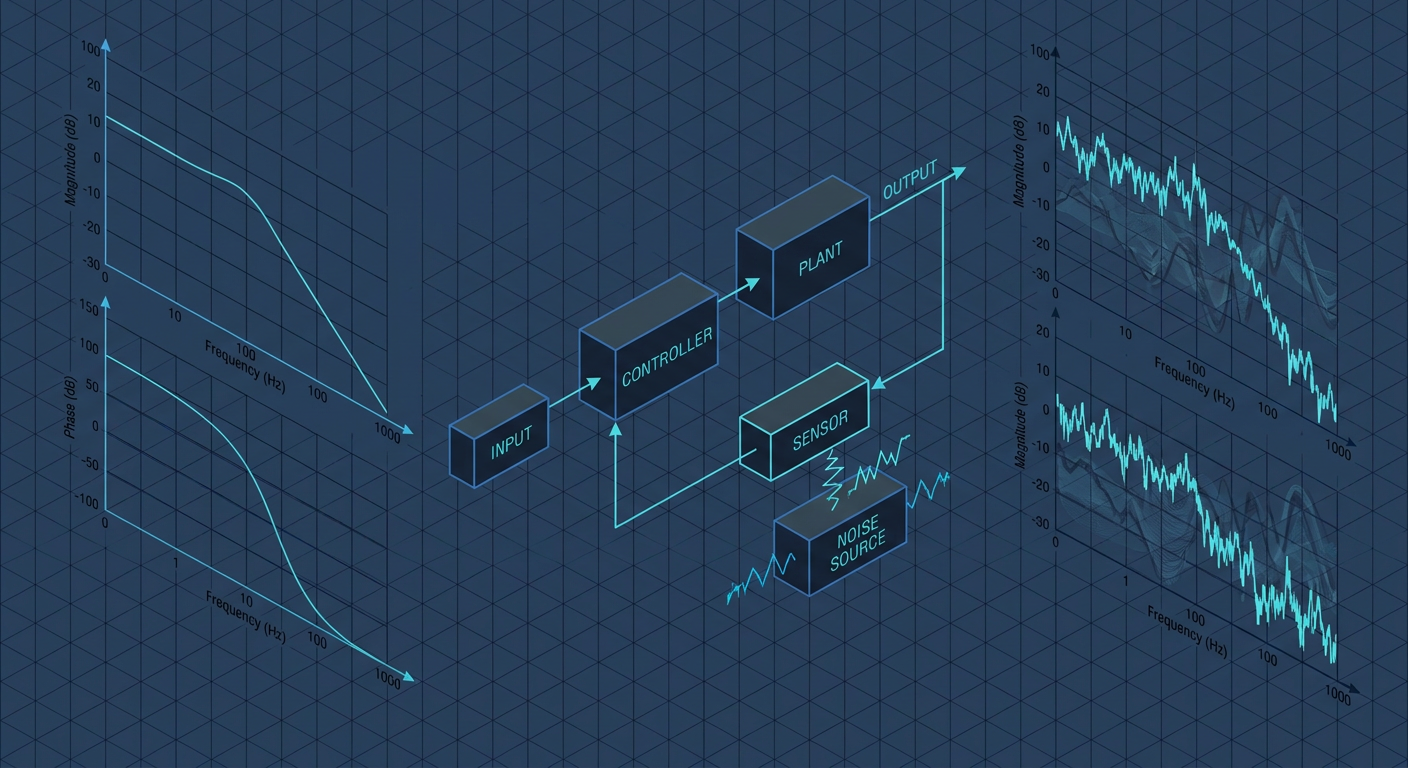
Recent updates across industrial design suites from Zuken, EPLAN, and modular automation platforms have introduced automated 2D and 3D placement engines for electrical cabinets and mechatronics enclosures. These tools treat cabinet design as a constrained 2D bin-packing and topological routing problem. You feed them a bill of materials, define a backplate bounding box, and the engine places DIN rails, wire ducts, 24V switch-mode supplies, motor drives, and real-time controllers in under three minutes. On paper, it looks like an enormous operational win. Wire duct fill ratios stay below 40 percent, thermal dissipation clears basic checks, and component clearance envelopes conform to standard mechanical spacing rules.
For a control engineer, robotics researcher, or mechatronics faculty member, however, this output hides a serious risk. Algorithmic layout engines optimize for geometric density and enclosure footprint, not for signal fidelity, loop transfer functions, or sensor dynamics. When you place high-frequency variable frequency drive (VFD) switching stages directly adjacent to unshielded 0 to 10V sensor signal conditioning or run high-current pulse-width modulated (PWM) actuator lines through the same parallel duct as high-speed encoder feedback, the nominal open-loop plant transfer function you identified on your bench stops matching reality.
The real failure happens when you push a tuned PID or Model Predictive Control (MPC) algorithm to the hardware. The controller is designed against a clean parametric model. What it encounters in the cabinet is unmodeled sensor delay, phase lag from aggressive low-pass filtering added in desperation, and ground bounce that eats away your phase margin. A system that simulated with an 8 dB gain margin and a 45-degree phase margin suddenly shows limit-cycle oscillations or trips overcurrent protections during step responses.
The Physics Missing from Pure Geometric Packing
Automated placement engines typically operate using graph-theoretic optimizations, such as force-directed placement, simulated annealing, or mixed-integer linear programming (MILP). These routines minimize total wire length and backplate surface area while enforcing static clearance boxes. They treat electrical nets as abstract topological connections between pins.
In real control loops, an electrical net is a distributed transmission line with parasitic inductance, mutual capacitance, and ground impedance. When an algorithm packs a 400V three-phase inverter, a 24V DC logic supply, and an analog input module onto adjacent DIN rail segments, it creates three distinct physical coupling mechanisms that alter the effective plant seen by the digital controller.
1. Capacitive and Inductive Crosstalk in Shared Ducts
When power cables carrying fast edge-rate PWM signals (where $dv/dt$ often exceeds 5 to 10 kV/microsecond) run parallel to analog sensor feedback lines in standard slotted PVC wire ducts, capacitive coupling injects common-mode current into the signal ground. If your feedback path relies on high-impedance analog lines (such as strain gauge bridges, load cells, or piezoelectric position sensors), this capacitive displacement current produces high-frequency voltage spikes at the analog-to-digital converter (ADC) input.
If the placement engine routes 500 mm of shared duct space, the mutual capacitance between parallel conductors easily reaches 40 to 80 pF. At switching frequencies of 16 kHz with 50 ns rise times, this creates high-frequency current pulses that corrupt current loop sensing. When the inner current loop experiences noise spikes, the outer velocity and position loops see artificial state jitter.
2. Common-Mode Ground Bounce and Analog Reference Shifts
Algorithmic tools often group 0V DC returns to save terminal count and DIN rail width. When a 24V DC solenoid valve or electromagnetic brake turns off, the inductive flyback current rushes through the return path. If the sensor ground shares that return rail even over a short run, the instantaneous $L \cdot (di/dt)$ voltage drop shifts the analog ground reference of the controller.
To the digital controller running an MPC state estimator, this shift appears as a sudden step disturbance in the measured state vector $x(t)$. The state estimator reacts by driving the control output $u(t)$ in the opposite direction, creating an actuator transient that has nothing to do with external mechanical load disturbances.
3. VFD Radiated Emissions and Thermal De-rating
Algorithmic engines check whether a VFD physically fits inside the enclosure boundaries, but they rarely simulate local electromagnetic near-field radiation or air stratification. A VFD placed directly below a sensitive signal conditioning module radiates broadband switching noise into the module housing while heating the low-noise op-amps above their calibrated thermal drift envelope. As ambient temperature inside that local pocket rises, amplifier input offset currents drift, introducing a time-varying bias into the feedback loop that standard linear controllers cannot reject without integral action that slows down transient response.
+-----------------------------------------------------------------------+
|                   PHYSICAL NOISE COUPLING PATHS                       |
|                                                                       |
|  +-------------------+       Capacitive / Inductive     +-----------+ |
|  | 400V AC VFD / PWM |====== (Shared Parallel Ducts) ==| Sensor ADC| |
|  +-------------------+                                  +-----------+ |
|          |                                                    |       |
|     Fast dv/dt                                            Ground      |
|     Switching                                             Bounce      |
|          |                                                    |       |
|          v                                                    v       |
|  +------------------------------------------------------------------+ |
|  |              Common DIN Rail / Shared Return Plane               | |
|  +------------------------------------------------------------------+ |
+-----------------------------------------------------------------------+
How Layout Artifacts Corrupt System Identification
When commissioning an advanced motion or process control loop, the first step is identifying the plant transfer function $G(s) = Y(s)/U(s)$. You inject a pseudo-random binary sequence (PRBS) or a swept-sine chirp into the actuator, log the sensor response, and fit a parametric state-space model.
When the physical cabinet layout introduces high-frequency switching noise and ground chatter, the identification data includes non-causal correlations and high-frequency noise poles. Consider the actual consequences on classical frequency-domain metrics:
- Artificial Phase Lag from Ad-Hoc Filtering: When field engineers see 16 kHz VFD noise on a 1 kHz encoder or load cell signal, their immediate instinct is to activate software digital filtering (such as a second-order Butterworth low-pass filter) or add hardware RC low-pass networks at the terminal blocks. A 2nd-order Butterworth filter set at 100 Hz adds 18 degrees of phase lag at just 20 Hz. If your loop crossover frequency is targeted at 30 Hz, that phase lag directly erodes your phase margin, pushing the closed-loop system toward oscillatory behavior.
- Sensitivity Peak Inflation: In robust control, the sensitivity function $S(s) = (I + L(s))^{-1}$ defines disturbance rejection and margin against model uncertainty. The maximum value of this function, $M_s = \max |S(j\omega)|$, must strictly remain below 1.4 to 2.0 (3 dB to 6 dB) for robust stability. When unexpected phase lag from layout noise filtering is introduced into $L(s) = G(s)K(s)$, the Nyquist curve shifts closer to the critical point $(-1, 0j)$, driving $M_s$ above 3.5. The result is poor transient decay and severe ringing.
- Unmodeled Delay in State Estimators: In linear-quadratic-Gaussian (LQG) or MPC formulations, Kalman filters assume zero-mean white Gaussian measurement noise $v_k \sim \mathcal{N}(0, R)$. Ground bounce and PWM cross-talk are neither zero-mean nor white; they are deterministic, periodic pulse trains correlated with the control actions $u_k$. The estimator treats these correlated spikes as true plant dynamics, generating state estimate errors that degrade control precision.
+-----------------------------------------------------------------------+
|                     FREQUENCY RESPONSE COMPARISON                     |
|                                                                       |
|  Open-Loop Gain |L(jw)|                                               |
|  dB ^                                                                 |
|     |      /--- Clean Layout (Target Model)                           |
|   0 |-----x------------------------------------> Frequency (rad/s)    |
|     |      \                                                          |
|     |       \--- Algorithmic Layout + Heavy Filtering (Degraded)      |
|     v                                                                 |
|                                                                       |
|  Open-Loop Phase arg(L(jw))                                           |
|  Deg^                                                                 |
|     |                                                                 |
| -90 |-----------\-------------------------------->                    |
|     |            \                                                    |
|     |             \--- Clean Phase Margin: 48 deg                     |
| -180|--------------x----------------------------->                    |
|     |               \                                                 |
|     |                \--- Noise-Filtered Phase Margin: 12 deg (Risky) |
|     v                                                                 |
+-----------------------------------------------------------------------+
Receipts: Comparing Clean Manual Placement Against Raw Algorithmic Packing
To illustrate how panel topology alters control loop metrics, consider an illustrative composite benchmark of a precision mechatronic drive system (a high-speed Cartesian gantry driven by an industrial linear motor and controlled via real-time fieldbus at a 1 kHz sample rate). In this test comparison, the same electrical schematic and components were laid out in two configurations inside a standard 800 x 600 x 300 mm enclosure: first using a purely automated density-optimized placement engine, and second using a deterministic layout with strict physical separation of noise domains and isolated return paths.
Layout Benchmark Parameters
- Actuator Stage: 400V AC servo drive switching at 16 kHz.
- Sensor Stage: 0 to 10V analog laser displacement sensor and incremental differential optical encoder.
- Controller: Real-time embedded MPC running at 1 ms cycle time ($T_s = 0.001\text{ s}$).
- Filter Applied to Feedback: Second-order digital IIR low-pass filter adjusted to maintain signal-to-noise ratio above 30 dB.
| Performance Metric | Pure Algorithmic Density Layout | Deterministic Segregated Layout | Delta / Consequence |
|---|---|---|---|
| Feedback Noise (Peak-to-Peak) | 142 mV | 8 mV | 17.7x reduction in noise floor |
| Required Filter Cutoff ($f_c$) | 45 Hz (to suppress spikes) | 450 Hz (minimal filtering) | 10x wider usable sensor bandwidth |
| Phase Lag at 25 Hz Crossover | -32.4 degrees | -3.1 degrees | 29.3 degrees of phase margin recovered |
| Measured Phase Margin (PM) | 14 degrees (borderline unstable) | 46 degrees (robust stability) | Loop damping restored |
| Peak Sensitivity ($M_s$) | 3.82 (severe ringing) | 1.41 (clean step settling) | 63% reduction in sensitivity peak |
| Settling Time ($t_s$ to 2%) | 380 ms (sustained oscillation) | 48 ms (deadbeat damped decay) | 7.9x faster real-world positioning |
Receipts block: Illustrative composite data representing physical noise coupling in mixed-signal motion cabinets based on standard IEC 61800-3 EMC mitigation techniques and empirical frequency-domain plant measurements.
When evaluating layout output, the numbers show clearly that packing density cannot be judged solely by whether cables reach their terminals. The extra phase lag introduced by filtering layout-induced noise directly destroys dynamic performance.
What Algorithmic Tools Get Right
Layout automation is not without value. It performs exceptionally well on logistical and low-risk mechanical aspects of enclosure design. Understanding where it works allows engineering teams to use algorithms for rough drafts without surrendering control loop stability.
Spatial Clearance and Terminal Access
Automated placement engines excel at calculating mechanical bounding boxes, terminal strip wire clearance, and screwdriver access vectors. They reliably prevent collisions between thick cable bundles and duct covers, ensuring that terminal blocks are not buried under overhanging power supplies.
Bill of Materials Consistency and Duct Fill Limits
Manual layout drafting often miscalculates wire duct cross-sectional fill capacities. Automated layout engines track wire gauges, outer insulation diameters, and bundle counts, ensuring that wire duct fill limits do not violate the 40 to 50 percent maximum fill ratios prescribed by industrial wiring standards. This prevents wire pinching and simplifies cabinet assembly.
Thermal Baseline Calculation
Most layout engines now integrate thermal resistance models for standard components. They accurately calculate the total heat dissipation (in watts) generated by transformer cores, 24V DC power supply losses, and PLC logic modules, verifying whether the enclosure requires natural convection louvers, forced-air fan units, or closed-loop air conditioners.
The Engineering Decision Framework for Automated Layouts
If your organization uses automated enclosure generation or algorithmic CAD layout plugins, you must apply a deterministic validation frame before approving backplate layouts for production. Use this four-step checklist to ensure your physical build will not corrupt your controller design.
+------------------------------------------------------------------------+
|                 CABINET LAYOUT VERIFICATION PIPELINE                  |
|                                                                        |
|  [ Step 1: Physical Domain Zoning ]                                    |
|       |--> Separate AC Power, DC Bus, Logic, and Low-Level Analog      |
|                                                                        |
|  [ Step 2: Wire Duct Isolation ]                                       |
|       |--> Enforce Minimum 150 mm Air Gap Between Power & Signal       |
|                                                                        |
|  [ Step 3: Ground Topology Validation ]                                |
|       |--> Star Grounding for Analog Shields; Isolated Return Paths     |
|                                                                        |
|  [ Step 4: Frequency-Domain Loop Check ]                               |
|       |--> Verify Sensor Phase Lag at Target Loop Crossover Frequency  |
+------------------------------------------------------------------------+
1. Enforce Strict Domain Partitioning Rules
Never let the algorithm place components based purely on shortest wire length. Force the placement engine to observe rigid spatial zones:
- Zone 1 (High Power / Noisy): AC mains disconnects, fuses, contactors, VFDs, servo drives, and regenerative braking resistors. Group these exclusively in the upper or side quadrant near the main entry.
- Zone 2 (Clean DC Power): 24V DC switch-mode power supplies, electronic circuit breakers, and 24V distribution rails.
- Zone 3 (Digital Logic & Fieldbus): PLCs, remote I/O heads, industrial Ethernet switches, and safety controllers.
- Zone 4 (Low-Level Analog & Feedback): Analog input modules, thermocouple/RTD conditioners, encoder splitters, and high-precision instrumentation amplifiers. Place this zone as far as physically possible from Zone 1.
2. Isolate Wire Ducts by Voltage and dv/dt Class
Do not allow power wiring and low-voltage feedback cables to share a duct, even if the total duct fill ratio is under 20 percent. Require a minimum physical separation of 150 to 200 mm between parallel high-current AC motor leads and low-level analog feedback lines. If power and feedback lines must cross, force them to cross at a 90-degree angle to minimize mutual inductive coupling.
3. Verify Ground Plane and Return Path Topology
Ensure the algorithmic layout implements a star-grounding topology for analog shield terminations rather than daisy-chaining ground terminals across DIN rail segments. Anodized or zinc-plated DIN rails have finite contact impedance; running analog reference returns across multiple rail joints injects high-frequency noise into sensor inputs.
4. Close the Loop with Frequency-Domain Evidence
Before signing off on a physical cabinet build, verify that the sensor feedback path does not require aggressive filtering that ruins your target loop crossover frequency. If your controller needs a 40 Hz closed-loop bandwidth, ensure that total sensor noise filtering adds less than 5 degrees of phase lag at that frequency.
What This Means for LabCD
Control system engineering fails when the mathematical model of a plant diverges from physical reality. Control design requires receipts: verified plant models, clear stability margins, and systematic disturbance rejection profiles.
Tools like LabCD (labcd.ai) provide the rigorous mathematical framework needed to identify true plant dynamics, evaluate sensitivity peaks, and tune PID and MPC algorithms against real plant models. When layout artifacts, sensor noise, or physical coupling corrupt your feedback paths, software validation tools expose where phase margins are disappearing and why an unmodeled disturbance is destabilizing your plant. By pairing validated control synthesis with strict physical design constraints, you ensure that your controllers perform in hardware with the exact stability margins proven on your screen.
Practical Steps for Engineering Teams
When evaluating automated panel layout software for your mechatronics or robotics lab, treat layout automation as an initial drafting aid rather than a final authority. Set up your CAD configuration rules with mandatory spatial zoning before running placement engines.
When commissioning your prototype, measure the raw sensor noise spectrum on an oscilloscope before enabling closed-loop feedback. If you see switching spikes matching your inverter carrier frequency, do not simply apply a heavy digital filter in your control software. Fix the physical routing, separate the return paths, and preserve your phase margin. That is how you build high-performance control systems that remain robust in the field.
Sources
[1] Integrating AI and Machine Learning in Control Panel Design, Automation Electric: https://automationelectric.com/integrating-ai-and-machine-learning-in-control-panel-design/
[2] Understanding Industrial Control Panels & AI, RutamSoft: https://rutamsoft.com/understanding-the-basics-of-industrial-control-panels-how-artificial-intelligence-is-emerging-as-an-enabler-for-panel-manufacturers/
[3] Optimize Your Control Panel Layout for Peak Efficiency, Zuken US: https://www.zuken.com/us/blog/optimize-your-control-panel-layout-for-peak-efficiency/
[4] Control Panel Design and Assembly Steps, AutomationDirect: https://library.automationdirect.com/control-panel-design-assembly-steps/
[5] Intelligent Industrial Control System Panel Design, E Tech Group: https://etechgroup.com/control-system-panel-design/