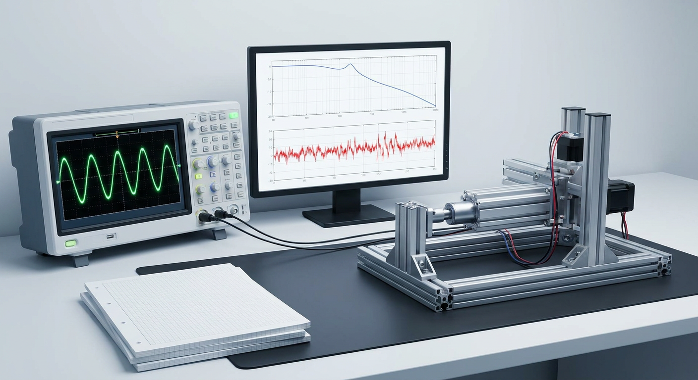
A recent debate across the control engineering community, highlighted on forums like r/ControlTheory, points to a clear fracture in how modern hardware teams model their plants. For decades, the standard path from an assembled electromechanical prototype to a tuned closed-loop controller ran through monolithic desktop software. An engineer collected a comma-separated data log, loaded a graphical system identification toolbox, clicked through interactive polynomial fitting menus, manually adjusted model orders, and exported a transfer function.
That workflow is breaking down on active production lines and agile mechatronics benches. Teams building custom brushless actuators, direct-drive robotic joints, precision gimbal stages, and fast-steering mirrors are increasingly ditching graphical desktop toolboxes. Instead, they write modular, headless system identification scripts in Python, Julia, or C++.
This shift is not driven by software ideology. It is driven by schedule risk, physical reality, and the need for repeatable evidence. When a robotics startup spins five prototype revisions of an integrated motor drive in three months, running manual curve-fitting sessions inside a licensed desktop application creates an unacceptable bottleneck. Worse, it produces plant models that conceal their high-frequency failure modes behind smooth graphical fits. Control engineers need pipelines that ingest raw swept-sine chirp telemetry, compute empirical transfer functions, isolate non-linear effects, and output verified linear state-space models with quantified uncertainty bounds in seconds.
The Friction of the Monolithic Desktop Toolbox
Commercial system identification suites, such as the legacy desktop toolboxes popularized over the past thirty years, are capable numerical packages. They contain mature implementations of subspace methods, prediction error minimization (PEM), and non-linear grey-box estimators. However, their architecture reflects an era when computing a plant model was an occasional, high-ceremony event performed by a dedicated specialist on a single workstation.
In modern mechatronics R&D, system identification must happen continuously. It runs across dozens of distinct physical units to capture manufacturing variance. It runs before and after thermal bake-out tests to quantify parameter drift. It runs inside automated continuous integration (CI) test suites to verify that firmware updates have not altered current-loop phase lag.
Desktop graphical interfaces introduce four distinct failure points into this cycle:
- Licensing and Headless Execution Barriers: Monolithic suites require dedicated seat licenses and heavy runtime environments. Running them on headless Linux continuous integration runners or embedded edge hardware during automated manufacturing end-of-line testing is expensive and operationally fragile.
- Opaque Preprocessing and Data Hygiene: Desktop interfaces encourage users to drag sliders for detrending, filtering, and reslicing data. When an engineer manually trims an unrepresentative transient by eye, they break reproducibility. If the identification routine cannot be re-executed identically from raw input logs via a single command, the resulting model cannot serve as a reliable baseline.
- Decoupling from the Embedded Firmware Pipeline: High-performance mechatronic controllers run on microcontrollers and real-time DSPs. When system identification lives in an isolated desktop program, transferring state-space matrices ($A, B, C, D$) or pole-zero cancellations back into embedded C code or modern simulation frameworks requires manual transcription, which introduces human error.
- Superficial Goodness-of-Fit Metrics: Standard desktop tools often highlight single-number fit percentages (such as normalized root mean square error). A 92% time-domain fit score looks reassuring in a slide deck, but it can hide a 180-degree phase discrepancy at the gain crossover frequency, guaranteeing that the physical feedback loop will oscillate once closed.
From Raw Chirps to Frequency Response Functions
To understand why scripted pipelines produce superior controllers, consider how an actuator plant must be characterized in the real world. A physical motor stage is never purely linear. It contains cogging torque, PWM inverter latency, encoder quantization noise, bearing stiction, and structural resonance modes from flexible couplings.
Raw Chirp / PRBS Input (u) ---> [ Physical Plant + Noise ] ---> Output (y)
                                            │
                                            ▼
                             [ Welch Averaging & Windowing ]
                                            │
                                            ▼
                          Empirical Transfer Function (ETFE)
                                            │
                       ┌────────────────────┴────────────────────┐
                       ▼                                         ▼
             Coherence Check γ²(f) > 0.8               Parametric Fit (SVD / N4SID)
                       │                                         │
                       ▼                                         ▼
            Isolate Noise / Non-linearities          Verified State-Space Model (A,B,C,D)
                                                                 │
                                                                 ▼
                                                    Uncertainty Bound Wm(s)
A custom identification script treats the characterization process as an automated pipeline. The experiment begins by injecting an excitation signal into the actuator's current or torque setpoint. While steps and square waves are simple, they concentrate energy in low frequencies and risk driving the mechanism into non-linear travel limits. Scripted workflows typically generate logarithmic swept-sine (chirp) inputs or carefully designed Pseudo-Random Binary Sequences (PRBS) that distribute excitation energy across the exact operational bandwidth of interest, typically from 1 Hz up to half the sample rate.
Once the input $u(t)$ and output $y(t)$ time series are logged, the scripted pipeline computes the Empirical Transfer Function Estimate (ETFE) using Welch's averaged periodogram method. The cross-spectral density $S_{uy}(f)$ and auto-spectral density $S_{uu}(f)$ are computed over overlapping windowed segments:
$$H(f) = \frac{S_{uy}(f)}{S_{uu}(f)}$$
Crucially, an automated script simultaneously computes the spectral coherence function:
$$\gamma^2(f) = \frac{|S_{uy}(f)|^2}{S_{uu}(f) S_{yy}(f)}$$
Coherence provides the first objective receipt of plant quality. If $\gamma^2(f)$ drops below roughly 0.8 at specific frequencies, the script immediately flags the data: the plant is either suffering from severe sensor noise, driving through a non-linear friction regime, or suffering from output clipping. A monolithic tool might still attempt to draw a smooth curve through these corrupted frequencies. A custom script automatically marks that band as invalid for parametric fitting.
Extracting Verified Continuous and Discrete Models
With a clean frequency response function (FRF) and validated coherence, the pipeline extracts low-order parametric models suitable for controller design, such as continuous-time transfer functions or discrete-time state-space representations:
$$x[k+1] = A x[k] + B u[k]$$ $$y[k] = C x[k] + D u[k]$$
Rather than relying on closed-box iterative optimizers that can get trapped in local minima, scripted pipelines often leverage deterministic subspace identification methods, such as N4SID (Numerical algorithms for Subspace State Space System Identification), or direct frequency-domain matrix fraction descriptions.
By executing a Singular Value Decomposition (SVD) on the block Hankel matrices constructed from input-output data, the script can inspect the decay of singular values. This provides a direct mathematical justification for selecting the model order. If the first four singular values capture 99.5% of the system's energy and the fifth drops by two orders of magnitude, the system order is objectively four: two states for rigid-body electromechanics and two states for the first torsional resonance mode.
No human guesswork is required. The script builds a fourth-order model, extracts the continuous poles and zeros, and maps them directly to physical system parameters: motor torque constant, total reflected rotor inertia, viscous damping, and shaft stiffness.
Illustrative Workflow Comparison
To illustrate the concrete engineering trade-offs between manual desktop modeling and scripted headless pipelines, consider an actuator characterization workflow across multiple prototype builds:
| Evaluation Metric | Manual Desktop Toolbox GUI | Scripted Automated Pipeline | Practical Engineering Consequence |
|---|---|---|---|
| Test Execution Time | 15 to 30 minutes per unit | Under 3 seconds per log | Custom scripts enable 100% end-of-line verification instead of random batch sampling. |
| Model Order Selection | Trial-and-error visual inspection | Singular value decay thresholding | Eliminates over-parameterization and spurious non-physical pole-zero cancellations. |
| Coherence Gating | Manual graph inspection | Automated masking where $\gamma^2(f) < 0.85$ | Prevents fitting controllers to unmodeled non-linear friction or sensor dropouts. |
| Pipeline Integration | Manual file export (.mat / .csv) | Native CI/CD API (JSON / C header generation) | Plant matrices ($A,B,C,D$) flow directly into firmware repositories without manual entry. |
| Uncertainty Quantification | Qualitative comparison plots | Explicit Multiplicative Error Bound $W_m(s)$ | Provides mathematical bounds for guaranteed closed-loop robust stability. |
Note: This comparison reflects a composite benchmark representative of high-throughput mechatronics development environments.
Quantifying Unmodeled High-Frequency Dynamics
Every physical plant model is an approximation. A linear model identified from actuator testbench data is generally valid only up to a specific frequency. Beyond that boundary, several physical effects destroy model fidelity:
- Phase lag introduced by anti-aliasing filters and digital computation delays ($e^{-s T_d}$).
- High-frequency structural modes, such as motor mounting bracket flexure or gear tooth compliance.
- Current loop saturation and back-EMF non-linearities at higher velocities.
Closing a high-gain feedback loop without defining where the model stops being trustworthy is the primary cause of instability in new mechatronics hardware. A controller designed against a pure second-order plant model will assume infinite phase margin at high frequencies, aggressively pumping control energy into mechanical resonance modes that the model ignored.
Custom identification scripts solve this by computing an explicit multiplicative uncertainty weight, $W_m(s)$, alongside the nominal plant $G_0(s)$. The script evaluates the difference between the empirical frequency response $G_{raw}(j\omega)$ and the identified parametric model $G_0(j\omega)$ across all measured frequency bins:
$$\Delta(j\omega) = \frac{G_{raw}(j\omega) - G_0(j\omega)}{G_0(j\omega)}$$
The script then fits a stable, minimum-phase upper bounding transfer function $W_m(s)$ such that:
$$|W_m(j\omega)| \ge |\Delta(j\omega)| \quad \forall \omega$$
Magnitude (dB)
      │
      │                                     /  Multiplicative Uncertainty Bound |Wm(jω)|
      │                                    /
      │                      ............./.... Unmodeled High-Frequency Dynamics
      │                     .            /
0 dB ─┼────────────────────.────────────/──────────────────────────────
      │  Nominal Plant    .            /
      │     |G0(jω)|     .            /     Trustworthy Plant Boundary
      │                 .            /      (Controller Gain Must Roll Off)
      └─────────────────┴───────────┴────────────────────────────────► Frequency (rad/s)
                                    ω_cross
This bounding function provides the exact stability limit for loop synthesis. According to the Small Gain Theorem, a feedback controller $K(s)$ designed for the nominal plant $G_0(s)$ will remain stable for all physical plant perturbations if and only if the complementary sensitivity function $T(s) = \frac{G_0(s)K(s)}{1 + G_0(s)K(s)}$ satisfies:
$$| W_m(s) T(s) |_{\infty} < 1$$
By generating $W_m(s)$ directly from data logs, the identification script hands the control engineer an indisputable constraint: a mathematically defined frequency ceiling beyond which loop gain must roll off. This prevents control engineers from artificially boosting loop bandwidth past what the physical hardware can sustain.
Synthesizing Closed-Loop Controllers with Validation Receipts
Once an accurate nominal model $G_0(s)$ and its uncertainty envelope $W_m(s)$ exist as programmatic objects, synthesizing and verifying a robust controller becomes deterministic. Whether deploying a classical PID with a second-order roll-off filter or a Model Predictive Controller (MPC) running on an embedded target, tuning moves from subjective bench tweaking to objective numerical verification.
A complete validation harness computes four core stability and performance receipts before firmware deployment:
- Vector Gain and Phase Margins: Classical gain and phase margins evaluate single-loop cuts, but they can overestimate stability if gain and phase fluctuate simultaneously. Scripted harnesses evaluate the peak sensitivity $M_s = |S(j\omega)|_{\infty}$, where $S(s) = (1 + G_0(s)K(s))^{-1}$. Keeping $M_s < 1.4$ to $1.6$ (approximately 3 dB to 4 dB) guarantees a minimum vector margin of at least $1/M_s$, preventing underdamped ringing.
- Disturbance Rejection Bandwidth: The script computes the sensitivity transfer function $S(s)$ to verify disturbance rejection. The frequency where $|S(j\omega)|$ crosses $-3\text{ dB}$ defines the disturbance rejection bandwidth, proving exactly what torque ripple and external load frequencies the closed loop can actively suppress.
- Control Effort and Actuator Saturation ($K S$): The transfer function from external output disturbance to actuator command, $K(s)S(s)$, is evaluated against the physical current limits of the motor drive. If a step disturbance command demands current higher than the thermal trip limit of the H-bridge inverter, the script rejects the tuning before hardware damage occurs.
- Cross-Validation on Fresh Data: The synthesized controller is simulated against independent validation data sets that were not used during the parameter estimation stage. If the simulated closed-loop response deviates from the validation dataset beyond a predefined error threshold, the model is flagged for revision.
What This Means for LabCD
For engineering teams building high-reliability mechatronics, controller tuning cannot rely on manual guesswork, unrepeatable GUI tweaks, or blind confidence in ideal mechanical CAD models. It demands control with receipts: an identified plant extracted from physical data, explicit bounds on unmodeled dynamics, and verified stability margins. Modern software must bridge the gap between low-level telemetry ingestion and rigorous mathematical synthesis.
LabCD is architected around this modern workflow. Instead of locking teams into heavy desktop interfaces, LabCD provides an automated, rigorous control workbench that combines continuous system identification, automated plant uncertainty bounding, and closed-loop PID and MPC design. It turns messy physical chirp telemetry into mathematically defensible state-space models and validated loop gains, giving control engineers the verifiable evidence they need before flashing code to real hardware.
A Practical Decision Frame for Hardware Teams
When evaluating whether to replace monolithic identification tools with a scripted identification pipeline on your team, use the following operational checklist:
- Prototype Iteration Velocity: If your mechanical or electrical hardware revisions cycle faster than once a month, manual desktop identification will delay firmware releases. Automate the ingestion of raw actuator chirps into parametric scripts.
- Fleet Variance and Calibration: If you produce more than ten physical units of an actuator mechanism, you cannot assume every motor matches nominal datasheet parameters. Use headless identification scripts to log parameter distributions (inertia, damping, torque constants) across every serial number.
- Safety-Critical and High-Bandwidth Demands: If your control loop operates near mechanical resonance frequencies or requires guaranteed settling times under disturbance, never rely on a simple time-domain curve fit. Enforce automated coherence checks and calculate the multiplicative uncertainty bound $W_m(s)$ to establish defensible gain crossover limits.
Systems behave according to their real physical dynamics, not our ideal assumptions. Replacing opaque desktop modeling steps with reproducible, automated system identification scripts ensures that your control loops are grounded in verified plant reality from the very first testbench run.
Direct Summary Q&A
Why are mechatronics teams replacing monolithic desktop system identification toolboxes with custom scripts?
Modern mechatronics workflows require continuous, automated, and repeatable modeling across multiple prototype builds and test runs. Custom scripts eliminate licensing bottlenecks, integrate directly with continuous testing and embedded firmware pipelines, and automatically calculate mathematically rigorous plant boundaries and uncertainty bounds that prevent closed-loop instability.