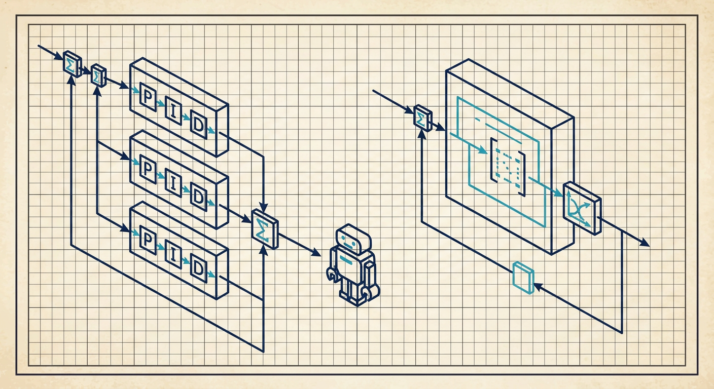
Dynamic robotic actuation has reached an uncomfortable architectural crossroads. Over the past twelve months, open-source trajectory libraries and compact quadratic programming solvers have made model predictive control (MPC) practical on embedded hardware. Research groups and industrial robotics teams are actively stripping out classical control cascades to run predictive solvers directly on their joint controllers.
The promise is obvious. MPC handles multi-variable cross-coupling, accounts for kinematic constraints natively, and respects hard voltage or torque limits before an actuator hits saturation. Yet in production runs and laboratory hardware validations, teams are hitting a familiar wall: solver execution jitter, unmodelled load changes, and non-deterministic recovery from infeasible states.
When a high-speed robotic arm strikes an unexpected obstacle or a quadruped leg slips on smooth concrete, a cascaded PID loop behaves predictably. It saturates, tracks error, and relies on anti-windup clamping. An embedded MPC solver running on a tight 1 millisecond control cycle can fail to converge within its allotted time budget. That leaves the firmware with two bad options: hold the previous control vector or push a sub-optimal step into the inverter.
For control engineers, faculty researchers, and mechatronics teams, choosing between cascaded PID and real-time MPC is not a matter of modern versus legacy tooling. It is a strict architectural trade-off involving compute budgets, plant identification accuracy, and safety validation requirements.
The Real-Time Constraint Budget
High-bandwidth robotic actuation demands fast feedback. In a field-oriented control (FOC) brushless powertrain, the inner current or torque loop typically executes between 10 kHz and 20 kHz directly on a microcontroller interrupt service routine. The velocity loop wraps around it at 1 kHz to 5 kHz, and the outer position loop runs between 500 Hz and 1 kHz.
Cascaded PID fits this hierarchy cleanly. Computing a single proportional-integral-derivative step requires a handful of multiply-accumulate operations. On an ARM Cortex-M7 running at 480 MHz, a complete three-tier cascaded loop with standard biquad filtering and feedforward terms computes in less than 3 microseconds. The execution time is perfectly deterministic. Every cycle takes the exact same number of clock instructions, making verification for hard real-time systems straightforward.
+-------------------------------------------------------------------------+
|                        CASCADED PID ARCHITECTURE                        |
|                                                                         |
|  Position Ref    +-------+  Velocity Ref  +-------+  Current Ref +-------+  Torque
| ---------------->| Pos P |--------------->| Vel PI|------------->|Cur PI |-------> Plant
|        ^         +-------+       ^        +-------+      ^       +-------+   |
|        |             |           |            |          |           |       |
|        +-------------+-----------+------------+----------+-----------+-------+
|                                 Feedback Signals (Encoders / Shunts)     |
+-------------------------------------------------------------------------+

+-------------------------------------------------------------------------+
|                         EMBEDDED MPC ARCHITECTURE                       |
|                                                                         |
|  State Trajectory   +---------------------------------------+  Optimal   Torque
| ------------------->| Convex Solver (OSQP / qpOASES / HPIPM)|  Control --------> Plant
|         ^           | Min Cost over Horizon N subject to:   |  Vector u[0]   |
|         |           |   x[k+1] = A x[k] + B u[k]            |                |
|         |           |   u_min <= u <= u_max                 |                |
|         |           |   x_min <= x <= x_max                 |                |
|         |           +---------------------------------------+                |
|         +-------------------------------|------------------------------------+
|                               State Feedback x[k]                        |
+-------------------------------------------------------------------------+
Model Predictive Control operates on a completely different mathematical footing. At each control step, the controller solves an online constrained optimization problem over a finite prediction horizon of $N$ steps. For linear MPC, this translates to a Quadratic Program (QP):
$$\min_{U} \sum_{k=0}^{N-1} \left( x_k^T Q x_k + u_k^T R u_k \right) + x_N^T P x_N$$
$$\text{subject to } x_{k+1} = A x_k + B u_k, \quad u_{\min} \le u_k \le u_{\max}, \quad x_{\min} \le x_k \le x_{\max}$$
Where:
- $x_k$ is the system state vector at horizon step $k$ (joint angle, angular velocity).
- $u_k$ is the control input vector (commanded torque or phase voltage).
- $Q, R, P$ are positive semi-definite weighting matrices defining performance priorities.
- $A, B$ represent the discrete-time linearised plant dynamics.
Even with highly optimised interior-point or active-set solvers like OSQP or qpOASES, solving this QP over a modest horizon ($N = 15$ to $N = 30$) requires hundreds of floating-point iterations. Execution time becomes variable. Depending on the initial state and how close the system is to its active constraint boundaries, the solver might converge in 150 microseconds or stall past 2 milliseconds.
If your control loop must deliver a deterministic torque update at 1 kHz, a solver that averages 400 microseconds but exhibits a worst-case execution time (WCET) of 1.4 milliseconds will cause missed deadlines, dropped packets, and limit cycles.
Where Actuator Saturation Breaks Assumptions
Actuator saturation is where the two control strategies diverge most sharply. Every physical motor has hard physical boundaries: maximum inverter phase voltage, thermal current limits, and peak bus current.
In a cascaded PID architecture, saturation is handled reactively using heuristic modifications. The most common is integral anti-windup: when the output stage hits its voltage limit, the integrator stops accumulating error. Velocity and acceleration feedforward terms help keep the error small during dynamic moves, but the controller remains blind to future limits. If a commanded motion trajectory demands more torque than the motor can produce, the joint falls behind the reference profile. The tracking error spikes, and the feedback loops overreact once the demand drops back within limits.
MPC handles boundaries proactively. Because constraints on states ($x$) and inputs ($u$) are baked directly into the optimization matrix, the solver knows about voltage and current boundaries across the entire prediction horizon $N$. If a fast deceleration is going to demand peak current three steps ahead, the optimizer begins trimming torque in advance, ensuring the joint glides precisely along the constraint boundary without overshoot.
This makes MPC dominant in multi-variable mechanisms where joints share dynamic couplings. A classic example is a dynamic robotic arm carrying a heavy payload, where accelerating joint one induces large reaction torques on joint two. A cascaded PID system sees these reaction torques purely as external disturbances. It must wait for the disturbance to deflect the joint before generating a corrective error signal. MPC incorporates the dynamic cross-coupling directly into its predictive $A$ matrix, adjusting joint two current the exact moment joint one begins its acceleration stroke.
Plant Identification and Model Sensitivity
The fundamental liability of MPC is its dependence on an accurate plant model. If the internal model $(A, B)$ does not match the actual hardware dynamics, predictive optimization loses its performance advantage. In severe cases of model mismatch, MPC performs worse than a simple PID controller.
Consider an industrial robotic joint experiencing temperature-dependent grease viscosity in its strain wave gearbox, combined with non-linear friction and rotor inertia variations. In a cascaded PID loop, gain margin and phase margin provide clear indicators of stability. A loop tuned with a 6 dB gain margin and a 45-degree phase margin can absorb significant variations in joint inertia and damping without losing stability.
Linear MPC provides no such direct frequency-domain guarantee out of the box. Robust MPC techniques can account for bounded parameter uncertainties, but they do so at the cost of heavier computation and conservative tracking performance. If the real joint contains unmodelled transmission compliance or cogging torque, the MPC solver will optimize a control trajectory for a fictional system, resulting in high-frequency chatter or steady-state tracking offsets.
+-------------------------------------------------------------------------+
|                     FREQUENCY DOMAIN VS OPTIMIZATION                    |
|                                                                         |
|  Cascaded PID / Classical               Model Predictive Control        |
|  ------------------------               ------------------------        |
|  - Gain Margin (e.g. > 6 dB)            - Weighting Matrices (Q, R, P)  |
|  - Phase Margin (e.g. > 45 deg)         - Prediction Horizon (N)        |
|  - Sensitivity Peak (M_s < 1.4)         - Linear Matrix Inqualities     |
|  - Robust to high-frequency dynamics    - Highly sensitive to unmodeled |
|    via low-pass biquad filtering          poles and delay variations    |
+-------------------------------------------------------------------------+
When a plant model is verified through rigorous system identification, MPC shines. When the model is estimated through crude approximations or theoretical CAD exports, deploying MPC on hardware becomes an exercise in endless solver debugging.
Architectural Comparison on Embedded Hardware
To understand the practical engineering trade-offs, examine how both approaches behave when implemented on representative mechatronic joint control hardware. The data below represents an illustrative composite based on embedded benchmarks running on an STMicroelectronics STM32H753 (ARM Cortex-M7 at 480 MHz, 32-bit floating-point unit) driving a permanent magnet synchronous motor (PMSM) through an 80:1 harmonic reducer.
Joint Controller Architecture Comparison
The metrics below represent an illustrative composite comparing standard cascaded field-oriented control with an embedded sparse active-set quadratic programming solver.
| Performance Metric | Cascaded PID + Feedforward | Linear Quadratic MPC (N=20) | Multi-Tier Hybrid (MPC over PID) |
|---|---|---|---|
| Current Loop Frequency | 20 kHz | N/A (Handled by inner loop) | 20 kHz (Hardware FOC) |
| Position/Velocity Rate | 1 kHz (Deterministic) | 500 Hz (Variable execution) | 200 Hz (MPC) / 20 kHz (FOC) |
| Mean Computation Time | 2.8 microseconds | 380 microseconds | 410 microseconds |
| Worst-Case Exec Time | 3.1 microseconds | 1,240 microseconds | 620 microseconds |
| Flash Memory Footprint | 14 kB | 185 kB | 196 kB |
| RAM Allocation | 2 kB | 48 kB | 52 kB |
| Actuator Limit Handling | Reactive (Anti-windup) | Proactive (Hard QP bounds) | Proactive Trajectory Limits |
| Tuning Parameters | 9 gains, 4 filter poles | 14 matrix weights, 2 horizons | 9 PID gains + 6 MPC weights |
| Disturbance Rejection | High (High gain margin) | Moderate (Model-dependent) | High (Combined structure) |
Notice the worst-case execution time (WCET) for standalone linear MPC. While its average computation time of 380 microseconds fits comfortably inside a 2-millisecond (500 Hz) frame, complex constraint interactions during sudden deceleration can push the solver past 1.2 milliseconds. If background communication tasks (such as EtherCAT or CANopen synchronous frames) interrupt the processor, the system risks violating its timing envelope.
This is why production robotics teams rarely run raw MPC down at the inverter gate level. Instead, they converge on the third column: a multi-tier hybrid architecture. A real-time predictive solver runs at a slower rate (100 Hz to 500 Hz) to optimize position, velocity, and torque trajectories within physical bounds, while a deterministic cascaded PID controller runs at high frequency (10 kHz to 20 kHz) to track those targets and reject high-frequency load disturbances.
Disturbance Rejection and Bandwidth Limits
Disturbance rejection in a robotic joint comes in two forms: low-frequency load changes (such as picking up an object of unknown mass) and high-frequency shock disturbances (such as a foot impact or mechanical backlash chatter).
Cascaded PID controllers excel at rejecting high-frequency disturbances because the inner loops run at extreme update rates. A current loop executing at 20 kHz with a closed-loop bandwidth of 1.5 kHz can suppress power supply ripple and torque cogging before the mechanical rotor has moved a fraction of a degree. The velocity loop, running at several kilohertz, uses derivative gain to inject immediate damping against mechanical impacts.
MPC struggles with high-frequency disturbance rejection when compute limits force its sample rate down. If an MPC loop runs at 250 Hz, its theoretical Nyquist frequency is 125 Hz, and its practical closed-loop disturbance rejection bandwidth is rarely higher than 25 Hz. If a dynamic disturbance hits the actuator faster than that bandwidth, the controller cannot generate an effective counter-torque until multiple sample periods have passed.
To improve disturbance rejection in MPC, engineers typically add disturbance observers (DOB) or augment the state space with an integrated disturbance state. While this eliminates steady-state tracking error, it adds more state variables to the QP, increasing solver iteration counts and worsening execution time jitter.
The Engineering Decision Frame
Selecting the right architecture comes down to five mechanical and computational constraints. Use this decision checklist during the initial controller design phase:
                     +---------------------------------------+
                     |  Does the mechanism have severe cross-|
                     |  axis coupling or hard state limits?  |
                     +---------------------------------------+
                                     /       \
                                   YES        NO
                                   /           \
     +----------------------------------+    +---------------------------------+
     | Can the MCU reliably solve a QP  |    | Use Cascaded PID + Feedforward. |
     | at >= 500 Hz with bounded WCET?  |    | Deterministic, high gain margin,|
     +----------------------------------+    | minimal RAM/Flash footprint.    |
                 /          \                +---------------------------------+
               YES           NO
               /              \
+------------------------+  +---------------------------------------------------+
| Deploy Embedded MPC.   |  | Deploy Multi-Tier Hybrid: MPC outer loop (100 Hz) |
| Verify plant model via |  | providing reference trajectories to deterministic |
| system identification. |  | high-speed Cascaded PID inner loops (20 kHz).     |
+------------------------+  +---------------------------------------------------+
1. Actuator Dynamics and State Coupling
If the robotic joint acts largely independently (such as a high-gear-ratio industrial SCARA joint where gearbox inertia dominates external link dynamics), cascaded PID with standard velocity and acceleration feedforward is simpler, safer, and faster to tune. If the system is lightly geared, direct-drive, or exhibits severe multi-axis dynamic coupling (such as humanoid balance or multi-link robotic arms), MPC provides tangible tracking benefits by optimizing the multi-variable input space.
2. Tightness of State and Input Constraints
When an actuation system must operate continuously at 95% of its thermal or voltage envelope without tripping inverter protection, MPC is superior. It plans trajectories that ride precisely on constraint boundaries without violating them. If the actuator has comfortable safety margins (operating at 60% to 70% of continuous ratings), PID anti-windup clamping is sufficient.
3. Compute Budget and Toolchain Verification
Running MPC requires a micro-solver compiled for embedded targets (such as C-code generated by ACADO, OSQP-Eigen, or CVXGEN) along with matrix algebra support. If the control hardware is an entry-level micro-controller with restricted RAM, the memory overhead and non-deterministic execution times make MPC a high-risk liability. If the hardware includes a dedicated real-time core (such as an ARM Cortex-R5 or Cortex-M7 with hardware double-precision floating-point), MPC becomes computationally viable.
4. Quality of System Identification
Never deploy MPC without a verified plant model. If the inertia matrix, friction curves, and motor transfer functions are rough estimates, the solver will produce erratic control vectors. If the team lacks the tooling or time to run rigorous system identification across operating temperatures, cascaded PID tuned with classical frequency-domain margins will be far more robust in the field.
5. Certification and Safety Verification
In medical, aerospace, and collaborative robotics applications, control firmware must often be validated against safety standards like IEC 61508 or ISO 13849. Proving stability and bounded response for a linear cascaded PID loop with classical gain and phase margins is established engineering practice. Proving worst-case execution time and asymptotic stability for an embedded numerical optimization solver under arbitrary sensor noise is difficult and expensive to defend in a design review.
What This Means for LabCD
Modern control engineering cannot rely on heuristic gain tweaking or unverified mathematical models. Whether implementing a high-bandwidth cascaded PID loop or an embedded predictive optimizer, engineers need verifiable proof that the control architecture stabilizes the physical plant across its entire operating envelope.
LabCD (labcd.ai) provides the analytical framework to bridge this gap. By combining system identification workflows with automated stability margin verification and controller synthesis, LabCD ensures that every control loop is backed by evidence. Rather than tuning gains by feel or guessing optimization weights, control teams can extract accurate continuous-time plant models, evaluate sensitivity peaks, verify disturbance rejection boundaries, and export validated control code. Whether your hardware demands the microsecond determinism of cascaded FOC or the proactive constraint handling of real-time MPC, LabCD gives you control with receipts.
Direct Architecture Selection Guide
Which control architecture is right for your robotic actuator?
- Choose Cascaded PID + Feedforward if your joint has high gear reduction, runs on resource-constrained microcontrollers, requires deterministic microsecond execution times, or must be verified using classical gain and phase margins.
- Choose Real-Time MPC if the actuator operates close to physical voltage and torque saturation limits, exhibits heavy multi-variable cross-coupling, and runs on an embedded processor capable of guaranteeing worst-case execution times within the sample budget.
- Choose a Multi-Tier Hybrid for high-performance dynamic robotics. Run a predictive optimizer at 100 Hz to 500 Hz to generate constraint-aware trajectory vectors, fed directly into deterministic 20 kHz cascaded current and velocity loops on the motor drive.
Watch your solver execution time distribution under edge-case load steps before committing to embedded MPC in production hardware. If the tail latency approaches your control period, move constraint handling to an outer loop and let classical cascades protect your hardware at the physical plant boundary.