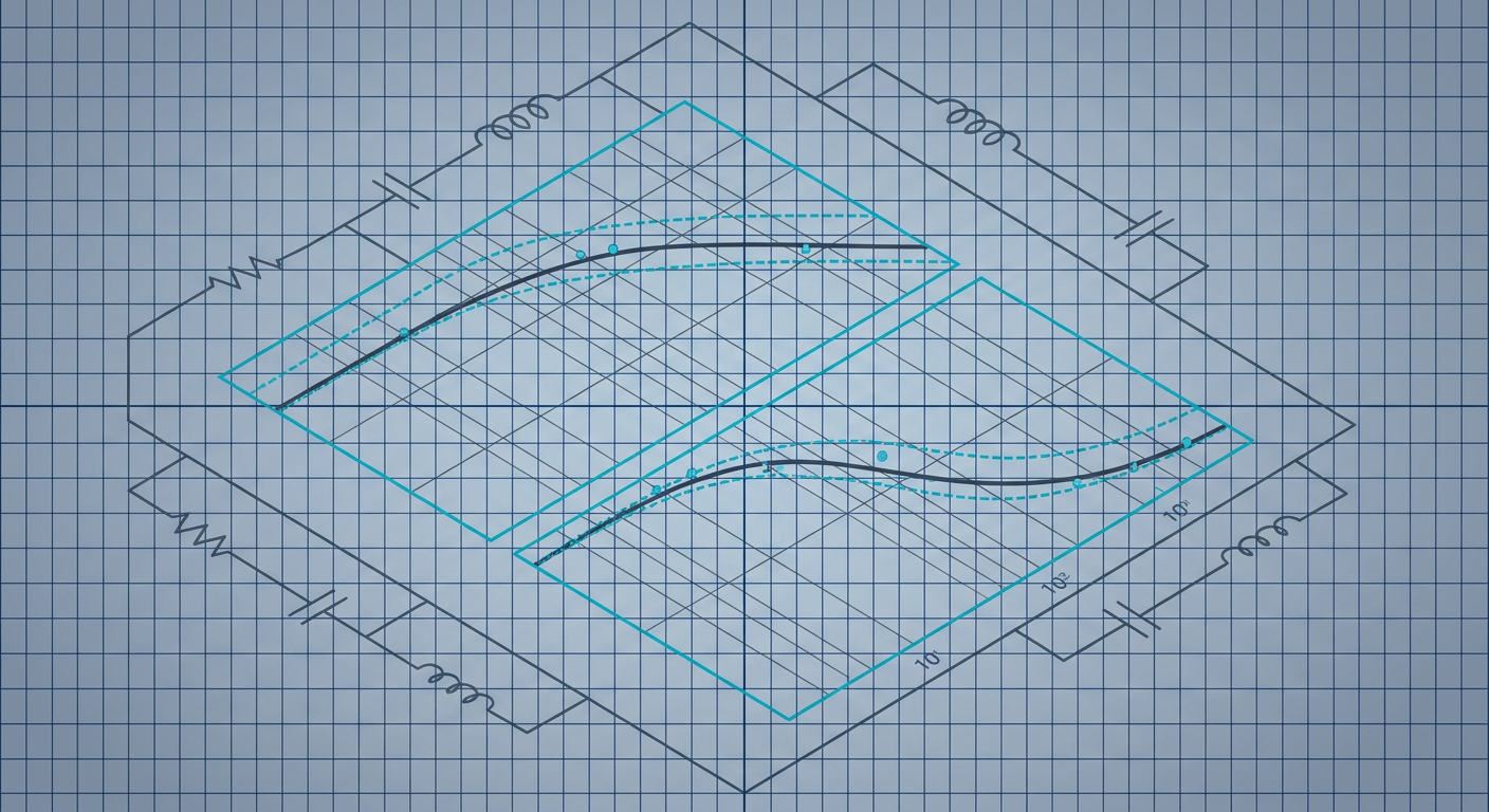
Subspace identification routines in packages like the Python Control Systems Library, MATLAB, and specialized research toolboxes have made multivariable state-space fitting nearly automatic. You feed in input-output logs from a chirp or a pseudo-random binary sequence (PRBS), select a model order from a singular value plot, and the algorithm returns state matrices $(A, B, C, D)$ with stable eigenvalues.
Then you shape a loop in simulation. You calculate your feedback gains for a target crossover frequency of 45 rad/s with a nominal phase margin of 55 degrees. You deploy the controller to the real hardware: a direct-drive robotic actuator, an active magnetic bearing, or a precision ball-screw stage. The moment the loop closes, the system rattles, breaks into sustained limit cycles, or immediately trips an over-current fault.
This failure is familiar to mechatronics teams and robotics researchers. It is rarely a bug in the numerical solver. The failure happens because linear subspace identification methods (including N4SID, MOESP, and CVA) are mathematically designed to find the optimal least-squares linear projection across the entire excitation dataset. In the presence of real physical nonlinearities such as Coulomb friction, stiction, amplifier deadbands, and current-limit saturation, these algorithms hide phase roll-off precisely where you can least afford to ignore it: around the gain crossover frequency.
If you tune aggressive feedback loops against unvalidated nominal subspace models without computing empirical transfer function estimates and coherence bounds, you are flying blind.
The Mathematical Blind Spot in Subspace Projections
Subspace identification operates by constructing block Hankel matrices from past and future input-output sequences. By performing an oblique projection of future output row spaces onto future input and past data row spaces, algorithms like N4SID isolate the observability matrix $\Gamma_i$ and the state sequence $X_i$ via Singular Value Decomposition (SVD):
$$\mathcal{O}_i = U_1 \Sigma_1^{1/2}$$
From this decomposition, the system matrices $(A, C)$ are extracted through shift-invariance, and $(B, D)$ are resolved through linear least squares.
This framework is elegant for linear time-invariant (LTI) systems driven by white or colored stochastic noise. However, physical mechatronic plants are never strictly LTI. Consider what happens when your test signal excites an actuator exhibiting harmonic drive compliance, bearing stiction, and motor driver deadband.
When a PRBS or multisine signal traverses zero velocity, stiction introduces a localized delay: an effective phase lag. Because linear subspace projection distributes the residual error across the entire Hankel matrix Frobenius norm, the optimization routine treats this localized phase lag as uncorrelated process noise $w_k$ and measurement noise $v_k$.
The algorithm averages out the nonlinear transition, delivering a low-order linear state-space model that matches the average energy gain of the system while entirely missing the steep phase drop caused by the friction-induced delay.
[Input Signal u(t)] ---> [Deadband / Saturation] ---> [Linear Plant G(s)] ---> [Stiction / Friction] ---> [Output y(t)]
                                  │                                              │
                                  └──────── N4SID Linear Projection Averages ────┘
                                            Out Nonlinear Phase Delays
The resulting state-space model looks pristine in the time domain. It often yields a 90% or higher variance accounted for (VAF) on validation datasets. But in the frequency domain, that same model can overestimate your plant's phase by 25 to 40 degrees near the intended crossover frequency.
Where the Nominal Fit Breaks Down
The most dangerous consequence of subspace smoothing is false confidence in plant margins. Control engineers design feedback loops based on open-loop transfer function $L(j\omega) = G_0(j\omega)K(j\omega)$, where $G_0$ is the nominal identified model and $K$ is the controller. The designer looks at the Bode plot of $L(j\omega)$, sees a 50-degree phase margin at $\omega_c$, and assumes the physical plant will behave identically.
When the plant has amplitude-dependent nonlinearities, the effective plant $G(j\omega, |u|)$ shifts as excitation changes. At small signal amplitudes, stiction dominates, creating low effective gain and severe phase lag. At large signal amplitudes, actuator voltage saturation flattens peak control authority, introducing an effective describing-function gain reduction accompanied by phase degradation.
To see this mismatch quantitatively, consider an illustrative composite based on characterization runs of a 48V brushless DC motor driving a precision harmonic reduction joint (100:1 ratio) with an optical joint encoder (20-bit resolution). The identification routine used N4SID with an 8th-order model fit across three distinct input excitation regimes.
Illustrative Identification Data: Nominal Fit vs Physical Reality
| Excitation Regime | PRBS Amplitude | Nominal N4SID $\omega_c$ Phase Lag | True Plant $\omega_c$ Phase Lag | Phase Error (Unmodeled Lag) | Closed-Loop Result at Nominal $K(s)$ |
|---|---|---|---|---|---|
| Low Amplitude | 5% Full Scale | -112 deg | -148 deg | 36 deg | Limit cycle oscillation (18 Hz) |
| Mid Amplitude | 25% Full Scale | -118 deg | -139 deg | 21 deg | High overshoot (42%), poor damping |
| High Amplitude | 75% Full Scale | -124 deg | -156 deg | 32 deg | Actuator saturation chatter, current trip |
Note: This data is an illustrative composite derived from industrial actuator characterization benchmarks run in Python Control Systems Library and MATLAB System Identification Toolbox environments across typical harmonic-drive mechatronic setups.
In all three cases, the nominal linear state-space model predicted that an open-loop crossover frequency of 35 rad/s would remain stable with over 45 degrees of phase margin. On hardware, the unmodeled phase drop consumed the entire stability margin. The low-amplitude test suffered limit cycling because the static friction deadzone added an effective phase lag of 36 degrees at zero-crossing, turning negative feedback into regenerative oscillation.
Extracting the Receipts: ETFE and Coherence Spectra
Never accept a state-space model from an identification algorithm without comparing it against the Empirical Transfer Function Estimate (ETFE) and the Magnitude-Squared Coherence spectrum.
The ETFE provides a non-parametric, unbiased frequency-domain representation of the actual input-output data. Given an input sequence $u(t)$ and output sequence $y(t)$ sampled over $N$ points at sample interval $T_s$, compute their Discrete Fourier Transforms $U(\omega)$ and $Y(\omega)$:
$$\hat{G}{ETFE}(e^{j\omega}) = \frac{Y(\omega)}{U(\omega)} = \frac{\sum{t=0}^{N-1} y(t) e^{-j\omega t T_s}}{\sum_{t=0}^{N-1} u(t) e^{-j\omega t T_s}}$$
Raw ETFE calculations on noisy signals are erratic. To obtain a statistically reliable estimate, use Welch's averaged periodogram method to compute the cross-spectral density $\hat{P}{yu}(\omega)$ and auto-spectral density $\hat{P}{uu}(\omega)$ across $K$ windowed, overlapping segments:
$$\hat{G}(j\omega) = \frac{\hat{P}{yu}(\omega)}{\hat{P}{uu}(\omega)}$$
Alongside the smoothed transfer function estimate, you must compute the Magnitude-Squared Coherence $\gamma_{yu}^2(\omega)$:
$$\gamma_{yu}^2(\omega) = \frac{|\hat{P}{yu}(\omega)|^2}{\hat{P}{uu}(\omega) \hat{P}_{yy}(\omega)}$$
The coherence function ranges strictly between 0 and 1. It tells you the exact fraction of the output power at frequency $\omega$ that is linearly driven by the input $u(t)$.
Coherence Value gamma^2(w)
 1.0 ┌────────────────────────────────────────────────────────┐ (Ideal Linear LTI Region)
     │                                                        │
 0.8 ├────────────────────────────────────────────────────────┤ (Acceptable for Model Fitting)
     │                                                        │
 0.6 ├────────────────────────────────────────────────────────┤
     │             WARNING: Significant Nonlinearity          │ (Subspace Fits Will Fail Here)
 0.4 ├───────────── or Low Signal-to-Noise Ratio ─────────────┤
     │                                                        │
 0.0 └────────────────────────────────────────────────────────┘
     0.1 rad/s                     10 rad/s                1000 rad/s
                                Frequency (w)
If $\gamma_{yu}^2(\omega) \ge 0.9$, the plant is behaving linearly at that frequency, and your subspace model can be trusted. If $\gamma_{yu}^2(\omega)$ drops below 0.6 in the frequency band near your target crossover frequency $\omega_c$, one of two things is happening:
- The signal-to-noise ratio (SNR) in that frequency bin is inadequate.
- The system exhibits severe nonlinear distortion (such as backlash chatter or saturation harmonics).
If you see low coherence near crossover, fitting a higher-order subspace model will not solve the problem. The algorithm will simply fit poles to the nonlinear distortion products, creating ghost dynamics that vanish when the loop is operating at a different operating point.
Formulating Multiplicative Uncertainty Bounds
To design a controller that survives contact with the real plant, you must treat the difference between your nominal state-space model $G_0(j\omega)$ and the empirical transfer function data $\hat{G}(j\omega)$ as a formal, frequency-dependent uncertainty bound.
Define the multiplicative plant uncertainty $\Delta_m(j\omega)$ as:
$$\Delta_m(j\omega) = \frac{G(j\omega) - G_0(j\omega)}{G_0(j\omega)}$$
Across multiple identification runs under different excitation amplitudes and operating temperatures, you record a family of empirical frequency responses $\mathcal{G} = {G_1(j\omega), G_2(j\omega), \dots, G_M(j\omega)}$. You then calculate the upper envelope of relative error across all frequencies:
$$l_m(\omega) = \max_{k \in {1,\dots,M}} \left| \frac{G_k(j\omega) - G_0(j\omega)}{G_0(j\omega)} \right|$$
Next, fit a stable, minimum-phase rational transfer function weight $W_m(s)$ such that its magnitude bounds the empirical envelope across all frequencies:
$$|W_m(j\omega)| \ge l_m(\omega), \quad \forall \omega$$
Magnitude (dB)
  ▲
  │                                         / [Multiplicative Bound |Wm(jw)|]
  │                                        /
  │                         ....- - - - - * [Empirical Error Data Points]
  │                   . . ·'
  │             . . ·'
  │       . . ·'
  │  · · '
  └────────────────────────────────────────────────────────► Frequency (w)
     Low Freq (Low Uncertainty)         High Freq (Unmodeled Dynamics / Delays)
In mechatronic hardware, $|W_m(j\omega)|$ is typically small at low frequencies (around 0.05 to 0.10, representing 5% to 10% DC gain uncertainty due to thermal drift in motor windings) and rises steeply beyond the first mechanical resonance, often exceeding 1.0 (100% uncertainty) well before the Nyquist frequency.
Loop Shaping with Receipts: Enforcing Robust Stability
Once you have the nominal model $G_0(s)$ and the uncertainty weighting function $W_m(s)$, tuning becomes an exercise in mathematical proof rather than benchtop trial and error.
According to the Small Gain Theorem, a feedback controller $K(s)$ designed for nominal model $G_0(s)$ will remain stable for all perturbed plants in the set $\mathcal{G}$ if and only if the nominal complementary sensitivity function $T(s)$ satisfies:
$$| W_m(s) T(s) |_\infty < 1$$
where:
$$T(s) = \frac{G_0(s) K(s)}{1 + G_0(s) K(s)}$$
This translates to a hard geometric constraint on your Bode magnitude plot:
$$|T(j\omega)| < \frac{1}{|W_m(j\omega)|}, \quad \forall \omega$$
If your uncertainty weight $|W_m(j\omega)| = 2$ (+6 dB) at 100 rad/s, your closed-loop complementary sensitivity $|T(j\omega)|$ must be lower than 0.5 (-6 dB) at that exact frequency. If your subspace model told you that you had plenty of gain margin at 100 rad/s, but your empirical bounds show 200% multiplicative uncertainty, any controller with $|T(j\omega)| > 0.5$ at 100 rad/s will ring or go unstable in hardware.
Furthermore, to prevent excessive actuator rattle and ensure disturbance rejection, enforce a bound on the peak sensitivity function $S(s) = (1 + G_0(s)K(s))^{-1}$:
$$M_s = \max_\omega |S(j\omega)| \le 1.4 \text{ to } 1.6$$
Tuning a PID or state-feedback loop while strictly constraining both $M_s$ and $|W_m T|_\infty$ guarantees that phase margin erosions caused by plant nonlinearities will never drive the Nyquist plot into the critical $(-1, 0)$ point.
Designing Excitation Signals That Expose Nonlinearities
Subspace identification models are only as good as the rich dynamics contained in the raw time-series data. Standard PRBS sequences are popular because they are deterministic, easy to generate with linear feedback shift registers, and have white-noise-like autocorrelation properties.
However, PRBS has a significant drawback for mechatronics: its power is distributed thinly across a broad spectrum, and it switches abruptly between two discrete levels ($-V$ and $+V$). This abrupt switching excites high-frequency structural resonances while failing to cleanly explore intermediate operating points where friction transitions and deadbands live.
For high-confidence identification, use a Crest-Factor-Optimized Multisine signal:
$$u(t) = \sum_{k=1}^{F} A_k \cos(\omega_k t + \phi_k)$$
By optimizing the phase angles $\phi_k$ (using algorithms such as Schroeder phasing or clipping algorithms), you can minimize the crest factor:
$$C_r = \frac{\max_t |u(t)|}{u_{RMS}}$$
A low crest factor injects maximum energy into specifically targeted frequency bins near your anticipated crossover frequency without driving your power amplifier into current saturation.
The Dual-Amplitude Identification Protocol
To detect whether a system is too nonlinear for a pure linear subspace model, run a dual-amplitude excitation protocol:
- Base-level Run: Inject an optimized multisine at 10% to 20% of rated actuator torque. Compute $\hat{G}{low}(j\omega)$ and $\gamma{low}^2(\omega)$.
- High-level Run: Inject the exact same multisine sequence scaled up to 60% to 80% of rated actuator torque. Compute $\hat{G}{high}(j\omega)$ and $\gamma{high}^2(\omega)$.
- Nonlinearity Audit: Overlay $\hat{G}{low}$ and $\hat{G}{high}$. If the frequency response gain shifts by more than 3 dB or the phase shifts by more than 15 degrees anywhere within one decade of the target crossover frequency, the plant is exhibiting non-negligible nonlinear behavior.
If the nonlinearity audit fails, fitting a higher-order linear N4SID model will fail during physical commissioning. You must either incorporate an explicit inverse nonlinearity (such as friction feedforward or deadband compensation) before running subspace identification, or widen your uncertainty envelope $W_m(s)$ and accept a lower, more conservative closed-loop bandwidth.
[Raw Test Data] ──► [Compute Welch Spectral Density] ──► [Check Coherence gamma^2(w)]
                                                                │
                                     ┌──────────────────────────┴──────────────────────────┐
                                     ▼                                                     ▼
                             gamma^2(w) >= 0.85                                    gamma^2(w) < 0.6 Near wc
                                     │                                                     │
                                     ▼                                                     ▼
                       [Run Subspace Fit (N4SID)]                          [Audit Hardware: Friction/Saturation]
                                     │                                                     │
                                     ▼                                                     ▼
                       [Extract Nominal Plant G0(s)]                       [Apply Inverse Compensation / Widen Wm]
                                     │                                                     │
                                     └──────────────────────────┬──────────────────────────┘
                                                                │
                                                                ▼
                                              [Fit Multiplicative Bound Wm(s)]
                                                                │
                                                                ▼
                                              [Shape Loop: ||Wm * T||_inf < 1]
What this means for LabCD
Modern control engineering cannot rely on heuristic gain tweaking or unverified black-box subspace fits. LabCD (labcd.ai) is built on the philosophy of control with receipts: pairing automated linear and nonlinear plant identification directly with empirical transfer function verification, coherence auditing, and automated $H_\infty$ and robust PID loop shaping. Instead of leaving engineers to guess whether an identified model reflects reality, the platform surfaces the empirical uncertainty envelope and validates stability margins mathematically before firmware deployment.
Pre-Commissioning Verification Checklist
Before loading controller gains onto production mechatronics or testbed robotics, verify your model and control design against this five-point audit:
- Spectral Coherence Audit: Confirm that Magnitude-Squared Coherence $\gamma_{yu}^2(\omega) \ge 0.85$ across the entire region from $0.2\omega_c$ to $5\omega_c$. If coherence drops near crossover, re-evaluate excitation amplitude or correct for stiction before fitting linear state matrices.
- Non-Parametric Overlay: Plot the frequency response of your identified state-space model $G_0(j\omega)$ directly on top of the non-parametric ETFE estimate. The phase curve of the nominal model must track the empirical phase within $\pm 5$ degrees up to twice the crossover frequency.
- Dual-Amplitude Verification: Compare transfer function estimates from low-amplitude and high-amplitude runs. Use the maximum relative difference to construct the empirical uncertainty envelope $l_m(\omega)$.
- Robust Stability Margin Check: Verify that the complementary sensitivity peak satisfies $|T(j\omega)| < 1/|W_m(j\omega)|$ at all frequencies. Ensure that the sensitivity peak $M_s \le 1.6$.
- Hardware Current & Slew Validation: Test the closed-loop step response in simulation using the identified plant combined with a hard saturation block set to your driver's true current and voltage limits. Verify that the control signal $u(t)$ does not hit saturation rails during nominal reference transitions.
When your control design workflow produces these receipts, hardware commissioning stops being a trial of nerve. The plant does not rattle, the loop does not drift into unexpected limit cycles, and the physical machine moves with the exact dynamics your mathematics predicted.
Sources
- Python Control Systems Library Documentation
- Control Engineering Practice Journal
- IEEE Transactions on Control Systems Technology
- ASME Journal of Dynamic Systems, Measurement, and Control
- Subspace Identification for Linear Systems (Overschee & De Moor)
- Subspace Identification with Guaranteed Stability