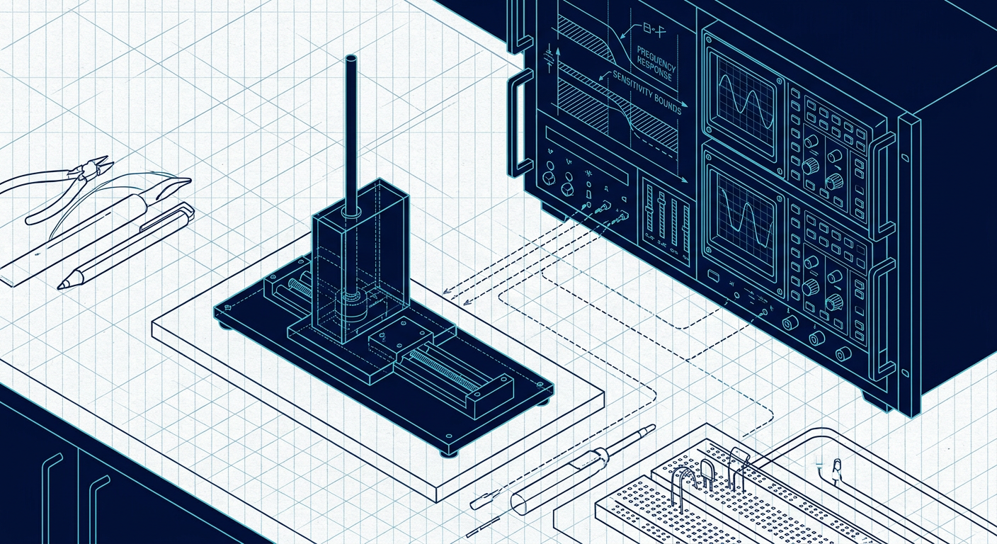
The IEEE Control Systems Society Technical Committee on Control Education recently published a community roadmap outlining why tertiary control training continues to produce graduates who struggle in practical mechatronics roles. The core issue is visible in almost every university laboratory across the world. A pair of students sits in front of a rotary pendulum or a DC motor test stand, turns three graphical sliders for proportional, integral, and derivative gains, watches the physical arm settle down after a step command, takes a screenshot of the clean oscilloscope trace, and pastes it into a lab report.
They receive full marks because the step response settled in under two seconds with less than five percent overshoot. Three months later, those same students join an industrial robotics team, deploy an identical gain-tuning philosophy to a dynamic joint actuator, and watch the system destroy its gearbox because unmodeled structural resonances and torque saturation triggered violent high-frequency limit cycles.
Treating control design as an empirical video game where students tweak numbers until the plant stops shaking teaches dangerous habits. It bypasses system identification, ignores loop transfer recovery, hides sensitivity peaks, and treats actuator saturation as a minor cosmetic inconvenience. To build engineers who can design flight controllers, precision motion stages, and industrial drives, universities and corporate training labs must replace black-box demonstrations with automated validation harnesses that grade controllers on mathematical robustness and plant uncertainty.
The Pathology of the Step Response Lab
The traditional undergraduate control curriculum splits cleanly into two incompatible halves. In the lecture hall, professors spend weeks covering the Nyquist stability criterion, root locus asymptotes, gain and phase margins, state-space pole placement, and Bode sensitivity integrals. In the laboratory, students run pre-compiled black-box routines or twist software potentiometers until the time-domain graph looks acceptable.
This disconnect creates a false sense of security rooted in three specific technical blind spots.
1. Blindness to Peak Sensitivity and the Waterbed Effect
When a student tunes a PID loop against a nominal second-order transfer function, they typically optimize for time-domain metrics: rise time, settling time, and peak overshoot. But time-domain step responses say almost nothing about robustness against out-of-band disturbances or high-frequency plant variation.
A controller can exhibit an apparently healthy phase margin of 45 degrees at its gain crossover frequency while harboring a massive sensitivity peak at an adjacent frequency. The sensitivity function $S(s) = (1 + L(s))^{-1}$, where $L(s) = G(s)K(s)$ is the open-loop transfer function, measures how disturbances and plant perturbations propagate into tracking error. If the peak sensitivity $M_s = \max_\omega |S(j\omega)|$ exceeds 2.0 (around 6 dB), the closed loop is dangerously close to the critical point $(-1, j0)$ on the Nyquist plane, even if the classical gain and phase margins appear nominally acceptable.
Under Bode's sensitivity integral, for any open-loop stable system with relative degree of at least two, the integral of $\ln |S(j\omega)|$ over all frequencies is zero:
$$\int_0^\infty \ln |S(j\omega)| , d\omega = 0$$
If a student forces aggressive disturbance rejection across low frequencies by driving the integral gain $K_i$ skyward without accounting for loop shaping, the sensitivity curve must pop up above unity elsewhere. In typical trial-and-error tuning, that amplification happens right at the plant's flexible modes or right above the Nyquist sampling limit. The step response looks calm because the input lacks spectral content at the peak frequency. The moment the physical system experiences a broadband torque disturbance or sensor quantization chatter, the closed loop rattles uncontrollably.
2. Ignoring Actuator Saturation and Integrator Windup
Most laboratory workstations shield students from physical non-linearities. The supplied software environments quietly clip current commands, clamp duty cycles, or insert hidden anti-windup algorithms inside pre-built blocks. The student never sees what happens when the error accumulates while the motor driver is hard against its voltage rail.
When these students design custom controllers from scratch, they write naive parallel PID structures:
$$u(t) = K_p e(t) + K_i \int_0^t e(\tau) , d\tau + K_d \frac{d e(t)}{dt}$$
During a large step change or an external hold, the integral state integrates the continuous error, pushing the calculated control effort $u(t)$ to ten times the motor driver supply rail. When the plant finally reaches the setpoint, the actuator remains pinned at full power until the error integrates in reverse. The result is massive overshoot, mechanical impact against end-stops, and burnt H-bridge drivers. If the laboratory software automatically manages this failure mode behind the scenes, the student learns nothing about back-calculation anti-windup, conditional integration, or actuator slew-rate limits.
3. Missing Plant Identification and Model Error Bounding
Real engineering design never starts with a clean transfer function like $G(s) = 5 / (s^2 + 2s + 5)$ handed down on a printed worksheet. Real engineering starts with an uncalibrated motor, an unknown friction profile, variable link inertia, and unmodeled sensor phase lag.
When academic labs provide exact transfer functions or rely entirely on trial-and-error manual tuning without system identification, students miss the most difficult phase of control engineering: determining the boundary where the mathematical model ceases to represent physical reality. They do not learn how to run swept-sine or chirp inputs, construct empirical transfer function estimates (ETFEs), extract coherence functions to identify non-linearities, or bound additive model uncertainties $\Delta(s)$ across frequency.
Automated Validation Bench: Illustrative Test Harness
To move away from qualitative lab reports, engineering programs are deploying open-hardware micro-pendulums, precision ballscrew stages, and dual-rotor aero systems connected to automated validation test suites. Instead of submitting a subjective paragraph explaining that the system seemed stable, the student commits their controller code (written in C, C++, or Python) to a test harness that compiles the control algorithm, flashes it to an embedded microcontroller, and subjects the physical plant to a battery of automated stress tests.
The harness executes calibrated multi-sine disturbances, injects synthetic sensor noise, steps the reference trajectory across linear and non-linear operating points, and records the closed-loop input-output data via high-speed hardware-in-the-loop (HIL) loggers.
The table below presents an illustrative composite benchmark comparing a typical trial-and-error student controller against a controller designed through identified plant dynamics, loop shaping, and anti-windup tracking on a precision inverted rotary pendulum rig.
| Performance and Robustness Metric | Target Spec | Student Trial-and-Error Loop | Validated Loop-Shaped Controller |
|---|---|---|---|
| Phase Margin ($PM$) | $\ge 45^\circ$ | $28.4^\circ$ (at $18.2\text{ rad/s}$) | $52.1^\circ$ (at $12.4\text{ rad/s}$) |
| Gain Margin ($GM$) | $\ge 6.0\text{ dB}$ | $3.8\text{ dB}$ | $9.6\text{ dB}$ |
| Peak Sensitivity ($M_s$) | $\le 1.6\text{ (4.1 dB)}$ | $2.85\text{ (9.1 dB)}$ | $1.42\text{ (3.0 dB)}$ |
| Complementary Sensitivity Peak ($M_t$) | $\le 1.25\text{ (1.9 dB)}$ | $1.92\text{ (5.7 dB)}$ | $1.15\text{ (1.2 dB)}$ |
| Settling Time ($2%$ Band, $10^\circ$ Step) | $\le 0.85\text{ s}$ | $0.62\text{ s}$ | $0.78\text{ s}$ |
| Overshoot under Nominal Conditions | $\le 10%$ | $4.8%$ | $6.2%$ |
| Overshoot with $+40%$ Arm Inertia | $\le 15%$ | $48.6%$ (Limit Cycle) | $11.4%$ |
| High-Frequency Noise Amplification ($>100\text{ Hz}$) | $\le 0.05\text{ A}_{RMS}$ | $0.34\text{ A}_{RMS}$ (Chatter) | $0.02\text{ A}_{RMS}$ |
| Recovery Time from 0.05 N-m Torque Hit | $\le 0.40\text{ s}$ | $1.15\text{ s}$ (Windup ring) | $0.28\text{ s}$ (Anti-windup clamped) |
| Automated Grading Verdict | Pass all gates | FAIL (Violates $M_s, GM, PM$) | PASS (Meets all receipts) |
Note: This data represents an illustrative composite benchmark derived from inverted pendulum hardware test setups running embedded digital controllers at a 1 kHz sample rate.
Looking at the nominal settling time and overshoot alone, the trial-and-error controller looks superior. It reaches the setpoint faster (0.62 seconds versus 0.78 seconds) and exhibits less overshoot (4.8 percent versus 6.2 percent). Under standard lab grading criteria, the trial-and-error controller would receive a higher score.
Under automated robustness validation, however, the trial-and-error controller fails completely. The high derivative gain amplifies encoder quantization noise into 0.34 A RMS of motor current chatter, heating the windings and chewing through gear teeth. Its peak sensitivity of 2.85 places it on the verge of instability. When the test rig applies a secondary clamp weight to simulate a 40 percent inertia mismatch, the trial-and-error loop enters a continuous non-linear limit cycle. The validated loop-shaped controller, designed with a sensitivity ceiling and proper low-pass derivative filtering, absorbs the parameter variation with minimal degradation.
Anatomy of an Automated Lab Grading Harness
Transitioning an engineering lab from manual inspection to automated verification requires three distinct subsystems: open hardware rigs with deterministic interfaces, a standard identification pipeline, and an asynchronous continuous-integration test runner.
+-------------------------------------------------------------+
|                   Student Controller Code                   |
|        (Pure C/C++ or MicroPython: State-Space / PID)        |
+-------------------------------------------------------------+
                              |
                              v
+-------------------------------------------------------------+
|                 Automated Test Harness (CI)                 |
|  - Static Code Analysis (No hidden bypasses, check timing)  |
|  - Flash to Microcontroller (STM32 / RP2040 / ESP32-S3)     |
+-------------------------------------------------------------+
                              |
                              v
+-------------------------------------------------------------+
|              Hardware Plant & Disturbance Injection         |
|  1. Baseline Nominal Step Tracking                          |
|  2. Swept-Sine Disturbance -> Calculate Empirical S(jw)     |
|  3. Solenoid Impact Hit -> Test Anti-Windup Recovery        |
|  4. Dynamic Switched Inertia -> Check Robust Stability      |
+-------------------------------------------------------------+
                              |
                              v
+-------------------------------------------------------------+
|                 Automated Metric Assessment                 |
|  [Pass/Fail] Ms <= 1.6 | PM >= 45 deg | Noise < Threshold   |
+-------------------------------------------------------------+
1. The Hardware Rig
Expensive closed-box industrial demonstration stations with proprietary USB drivers are being phased out in favor of open-hardware mechatronics platforms. A modern bench setup consists of an off-the-shelf brushless motor with field-oriented control (FOC), an absolute magnetic or optical encoder with at least 14 bits of resolution, an auxiliary disturbance actuator (such as a small voice coil or a switched friction brake), and a standard microcontroller board (such as an STM32G4, RP2040, or ESP32-S3).
Because the hardware bill of materials is low, universities can deploy dozens of identical benches or allow students to take them home as portable lab kits. The key requirement is determinism: the firmware running the low-level loops must sample sensors and update PWM outputs at a fixed interval (typically 1 kHz to 10 kHz) with minimal jitter.
2. The Model Identification Phase
Before students are permitted to write a single line of control logic, they must generate an identified linear model with quantified uncertainty bounds.
The student writes an identification script that commands the actuator to inject a zero-mean pseudo-random binary sequence (PRBS) or a logarithmic chirp across a specified bandwidth (for example, 0.1 Hz to 200 Hz). The test harness records the input current and output angular velocity, computes the cross-spectral density, and calculates the empirical transfer function estimate along with the coherence function $\gamma_{xy}^2(\omega)$:
$$\gamma_{xy}^2(\omega) = \frac{|S_{xy}(j\omega)|^2}{S_{xx}(\omega) S_{yy}(\omega)}$$
If the coherence drops significantly below 0.8 within the target control bandwidth, the student cannot proceed to synthesis until they address non-linearities, friction deadbands, or poor excitation levels. Once a reliable transfer function $G(s)$ is fitted, the student extracts an additive uncertainty bound $W_m(s)$ such that the true plant $G_p(s)$ satisfies:
$$G_p(s) = G(s)(1 + W_m(s)\Delta(s)), \quad |\Delta|_\infty \le 1$$
3. The Continuous Integration Test Pipeline
When the student finishes designing their controller, they push their controller repository to a local campus Git server or plug into the physical lab station's USB testing harness. The automated pipeline performs a three-stage verification process:
- Static Analysis and Compilation: The harness checks that the code conforms to hard real-time execution constraints, contains no dynamic memory allocations inside the control loop, and includes anti-windup clamping logic.
- Hardware-in-the-Loop Nominal Validation: The compiled binary runs on the physical hardware. The harness commands a standard setpoint profile and logs error, control effort, and execution jitter.
- Robustness and Disturbance Injection: The harness triggers the auxiliary disturbance mechanism. It injects a calibrated current pulse into the motor while simultaneously commanding a step transition. It then runs a multi-frequency test signal to directly measure the sensitivity function $S(j\omega) = e(j\omega) / r(j\omega)$ across the crossover region.
If the controller violates any hard constraint, such as $M_s > 1.6$, peak current exceeding the thermal limit, or steady-state error failing to clear within the allocated timeframe, the harness rejects the submission and provides the exact Bode and Nyquist plots showing where the stability margin broke down.
Practical Decision Frame for Control Educators and Team Leads
Building an automated validation lab requires shifting instructional priorities away from qualitative visual observation and toward verified bounds. Whether upgrading an academic mechatronics curriculum or restructuring internal training for a robotics engineering department, use the following operational checklist.
1. Abolish Unconstrained Step Response Grading
Never grade a student or junior engineer solely on settling time and overshoot from an undisturbed step command. An aggressive, fragile loop will always beat a robust loop on a clean step response. Introduce compulsory multi-frequency disturbance injection and require students to report sensitivity peak ($M_s$) and complementary sensitivity peak ($M_t$) alongside time-domain metrics.
2. Force Explicit Anti-Windup Implementation
Disable built-in, pre-packaged anti-windup blocks in your simulation and hardware environments. Require students to write the integrator clamping, back-calculation, or conditional integration logic directly in code. Test this explicitly by injecting an external mechanical block that holds the actuator static for two seconds during an active step command, then releasing the block and logging the transient recovery.
3. Implement Plant Perturbation Testing
Every laboratory rig should support mechanical or electrical variations that can be switched in seconds. Examples include magnetic attachable flywheels that double the rotor inertia, switchable eddy-current dampers, or variable-rate springs. A controller is only valid if it maintains stability and meets performance bounds across the full range of plant variations without retuning.
4. Provide Real Receipts Over Subjective Reports
Replace thirty-page narrative lab reports with standardized validation sheets generated automatically by the test harness. The report should display the identified plant model, the measured sensitivity function, the time-domain disturbance response, and pass/fail verdicts against defined margins.
What This Means for LabCD
Modern control engineering cannot rely on manual trial-and-error tuning or unverified assumptions about plant behavior. LabCD (labcd.ai) provides the core engine for this workflow, connecting direct system identification, automated stability margin calculation, and loop shaping into an integrated software pipeline.
Instead of leaving engineers to guess whether their controller will hold up under real-world plant variations, LabCD computes the exact sensitivity peaks, robust stability margins, and anti-windup requirements against identified models. The platform turns control design from an empirical guessing game into a rigorous engineering discipline backed by verifiable mathematical receipts.
Moving from Demonstration to Verification
The fundamental goal of control education is not to demonstrate that a feedback loop can stabilize a pendulum under pristine conditions. The goal is to teach engineers how to construct feedback systems that remain safe, predictable, and robust when every assumption about the physical world begins to degrade.
By replacing black-box demonstration software with open hardware and automated validation pipelines, engineering programs can bridge the gap between abstract control theory and the brutal realities of hardware implementation. When students are forced to defend their loops with phase margins, sensitivity bounds, and anti-windup receipts, they stop being slider-tweakers and start operating as true control engineers.
Sources
[1] Quanser Control Education Hardware Systems: https://www.quanser.com/products/
[2] IEEE Control Systems Society Technical Committee on Control Education: https://www.ieeecss.org/technical-committee/control-education
[3] Control Education for Societal-Scale Challenges: A Community Roadmap: https://www.sciencedirect.com/science/article/pii/S1367578823000111
[4] IFAC Technical Committee on Control Education Resources: https://www.youtube.com/playlist?list=PLLhem8_dLoapbRvc-jtYj1JDIUsTvJX4o
[5] A Survey of Algorithms for Black-Box Safety Validation of Cyber-Physical Systems: https://www.jair.org/index.php/jair/article/view/12716
[6] PID Controller Theory, Tuning Methods, and Loop Robustness: https://en.wikipedia.org/wiki/PID_controller