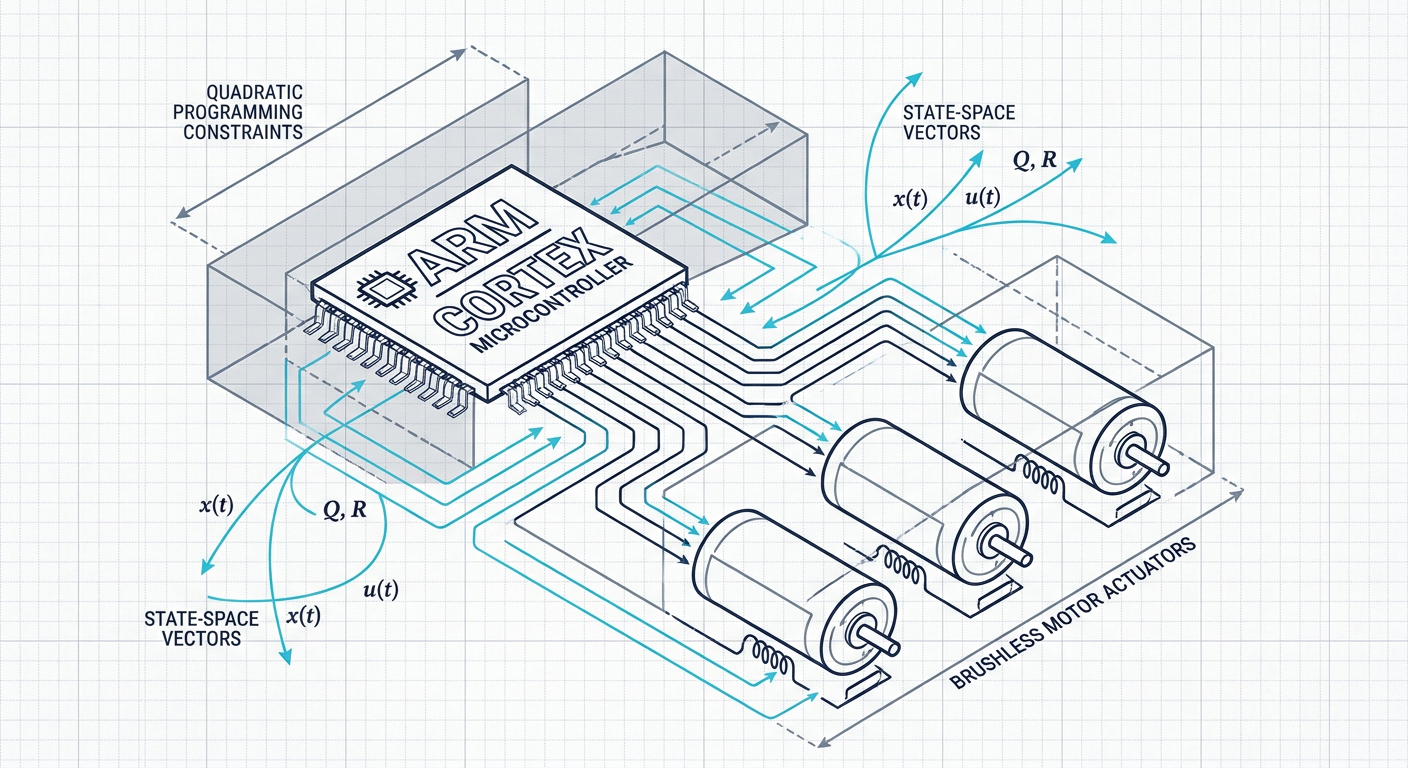
Embedded control engineers have spent decades treating Model Predictive Control (MPC) as the exclusive domain of Linux single-board computers. If you wanted to solve a constrained quadratic program at hundreds of hertz, you had to budget for an auxiliary compute module like an NXP i.MX8 or an NVIDIA Jetson. You accepted the added bill of materials, the three-watt power penalty, and the thermal headaches that come with running an operating system next to an inertial measurement unit.
The release and robotics validation of TinyMPC, developed by researchers at Carnegie Mellon University and partner labs, breaks that constraint. By reformulating the alternating direction method of multipliers (ADMM) to exploit linear time-invariant dynamics, TinyMPC shrinks memory footprint down to tens of kilobytes of Flash and pushes execution times well below 500 microseconds on a standard 168 MHz ARM Cortex-M4F. Hardware tests on platforms like the Bitcraze Crazyflie show that high-rate, multi-variable, constrained optimization can run directly inside the primary microcontroller's real-time loop.
For engineers designing camera gimbals, micro-drones, precision actuators, and robotic end-effectors, this shift changes the economics of control. You no longer have to pick between brittle anti-windup PID heuristics and expensive companion computers. You can enforce hard voltage, torque, and kinematic constraints directly on budget silicon.
The Memory and Compute Wall of Embedded Solvers
Traditional embedded quadratic programming (QP) solvers hit three hard walls on low-cost microcontrollers: dynamic memory allocation, matrix factorization overhead, and predictable execution budgets.
Consider a standard dense or sparse convex quadratic program derived from a linear discrete-time state-space model:
$$\min_{x, u} \frac{1}{2} \sum_{k=0}^{N-1} \left( x_k^T Q x_k + u_k^T R u_k \right) + \frac{1}{2} x_N^T Q_N x_N$$
$$\text{subject to } x_{k+1} = A x_k + B u_k, \quad u_{\min} \le u_k \le u_{\max}, \quad x_{\min} \le x_k \le x_{\max}$$
Where $x_k \in \mathbb{R}^n$ represents the state vector, $u_k \in \mathbb{R}^m$ represents the control input, and $N$ is the prediction horizon.
General-purpose convex solvers such as OSQP or qpOASES solve this problem reliably on desktop processors. On an ARM Cortex-M4 or Cortex-M7, however, their generalized linear algebra routines require significant RAM for working variables and workspace buffers. A typical OSQP formulation for a 12-state, 4-input quadrotor over a 20-step horizon can consume tens of kilobytes of dynamic heap space. On a microchip with 64 KB to 192 KB of total SRAM shared with RTOS stacks, motor commutation routines, and telemetry buffers, that memory footprint is unacceptable.
Linear system solves represent the primary compute bottleneck. Standard operator splitting methods require solving a linear system of the form $(H + \rho A^T A) z = v$ at every inner iteration, where $H$ is the Hessian, $A$ is the constraint matrix, and $ ho$ is the penalty parameter. When constraints change or step sizes adapt dynamically, the solver must continuously factorize large, sparse matrices or perform expensive forward and back substitutions. On an integer-heavy Cortex-M4 core without double-precision hardware acceleration, these algebraic steps stall the processor.
When a control loop misses its deadline because an interior-point solver required 45 iterations instead of 8 to converge, the actuator drops its packet, phase margin vanishes, and the physical plant destabilizes.
How TinyMPC Compresses the Linear Solve
TinyMPC resolves the compute bottleneck by changing how the optimization problem is structured before code generation occurs. It exploits a property often ignored by generic mathematical programming tools: for linear time-invariant (LTI) systems, the plant matrices $A$ and $B$, the cost weights $Q$ and $R$, and the horizon length $N$ remain constant across time steps.
Instead of treating dynamic balance constraints $x_{k+1} = A x_k + B u_k$ as general affine constraints alongside actuator limits, TinyMPC enforces the system dynamics directly through an unconstrained Riccati-like linear solve within the ADMM splitting scheme. It decouples the state and input variables into two alternating update steps:
- A primal linear quadratic tracking subproblem that satisfies the system dynamics over the horizon $N$.
- A projection subproblem that clips state and actuator bounds element-wise.
Because the dynamics and cost matrices do not change online, the matrix requiring inversion in the primal step is constant. TinyMPC computes its Cholesky or Riccati factorization offline on the host computer. The embedded target stores only the pre-factored matrices in read-only Flash memory.
During runtime execution on the Cortex-M4, the linear solve reduces to simple matrix-vector multiplications and vector additions. The projection step reduces to element-wise operations:
$$z_k = \text{clamp}(u_k + \sigma_k, u_{\min}, u_{\max})$$
No heap allocations take place. No matrix factorizations occur inside the interrupt service routine. The solver executes in deterministic, static memory with predictable cycle counts per iteration.
Receipts: Memory and Execution Benchmarks
To understand what this architectural change yields on real silicon, we examine benchmark data from the TinyMPC ICRA publication across standard robotics test cases running on bare-metal and RTOS-governed ARM Cortex-M microcontrollers.
Embedded Solver Footprint and Solve Time Benchmarks
Setup: Benchmarks compiled with GCC with -O3 optimization, executing trajectory tracking for a 12-state, 4-input multirotor system over a prediction horizon of $N = 10$. Target hardware: STM32F405 (ARM Cortex-M4F at 168 MHz) and Teensy 4.1 (ARM Cortex-M7 at 600 MHz). Data source: Nguyen et al., ICRA 2024 TinyMPC publication.
| Solver | Target Processor | Clock Speed | Flash Footprint | Peak RAM | Avg Solve Time | Max Solve Time |
|---|---|---|---|---|---|---|
| OSQP (Sparse) | STM32F405 (M4F) | 168 MHz | ~42 KB | ~18 KB | 4,210 µs | 11,800 µs |
| TinyMPC | STM32F405 (M4F) | 168 MHz | ~9.5 KB | ~2.1 KB | 380 µs | 610 µs |
| OSQP (Sparse) | Teensy 4.1 (M7) | 600 MHz | ~42 KB | ~18 KB | 820 µs | 2,450 µs |
| TinyMPC | Teensy 4.1 (M7) | 600 MHz | ~9.5 KB | ~2.1 KB | 78 µs | 135 µs |
On the Cortex-M4F running at 168 MHz, TinyMPC drops the average solve time from 4.2 milliseconds to 380 microseconds. This speedup is the difference between being trapped at a sluggish 50 Hz control rate and running a fully predictive, constrained 500 Hz inner loop on standard drone and gimbal flight controllers.
[ Trajectory / Setpoint Reference ]
                │
                ▼
┌──────────────────────────────────────────┐
│         ARM Cortex-M4 / Cortex-M7        │
│                                          │
│  ┌────────────────────────────────────┐  │
│  │        TinyMPC Core Loop           │  │
│  │                                    │  │
│  │  1. Primal Riccati Solve (Flash)   │  │
│  │     Static pre-factored matrices   │  │
│  │     Time: ~180 µs                  │  │
│  │                                    │  │
│  │  2. Dual Box Clamping (SRAM)       │  │
│  │     Hard bounds [vmin, vmax]       │  │
│  │     Time: ~40 µs                   │  │
│  │                                    │  │
│  │  3. Convergence Residual Check     │  │
│  │     Fixed max-iteration guard      │  │
│  └────────────────────────────────────┘  │
└─────────────────────┬────────────────────┘
                      │
                      ▼
          [ Actuator PWM / FOC ]
The Engineering Payoff: Enforcing Hard Dynamic Limits
Why go through the effort of deploying MPC on a microcontroller when cascaded PID is already well understood and executes in under five microseconds?
The practical answer lies in multivariable constraint handling. Cascaded PID handles actuator saturation poorly because each loop acts in isolation. Consider a direct-drive three-axis brushless gimbal stabilizing an optical payload under abrupt base disturbance.
In a cascaded architecture, the outer velocity loop requests a corrective torque from the inner current loop. If the motor reaches its maximum continuous current or supply voltage limit, the integrator begins to wind up unless explicitly clamped. If cross-axis coupling introduces gyroscopic torque from a rapid yaw maneuver, the pitch axis controller has no knowledge that the yaw axis is already consuming the entire battery bus current margin. The axes fight each other, phase margin degrades, and the image blurs.
Under TinyMPC, dynamic cross-axis coupling and physical boundaries enter the formulation as explicit linear bounds:
- Voltage and Current Limits: $u_{\min} \le u_k \le u_{\max}$ prevents the field-oriented controller (FOC) from requesting phase voltages outside the linear modulation region of the inverter.
- Joint Travel and Mechanical Stops: $x_{\min} \le x_k \le x_{\max}$ keeps lens assemblies away from physical bumper stops without relying on soft software dampers that degrade tracking bandwidth.
- Angular Velocity Slew Rates: $\Delta u_{\min} \le u_k - u_{k-1} \le \Delta u_{\max}$ caps the rate of torque change, suppressing high-frequency mechanical resonance in lightweight structural carbon fiber.
Because the optimizer evaluates these constraints across the prediction horizon, it starts braking before the gimbal hits an operational limit. It prioritizes axes based on the cost weighting matrix $Q$. If keeping roll level is mission-critical while yaw error is acceptable, the optimizer automatically sacrifices yaw tracking to keep roll within its strict constraint bounds.
Where Small Solvers Break Down: Model Mismatch and Latency
TinyMPC is not magic. It trades algorithmic generality for raw execution speed and tiny memory footprints. When implementing this class of solver on real hardware, mechatronics teams must navigate three distinct failure modes.
1. The Preconditioner Rigidity Trap
TinyMPC derives its performance from offline matrix factorization. If the physical plant parameters drift significantly during operation, the precomputed Cholesky and Riccati matrices stored in Flash become inaccurate.
If you tune TinyMPC for a quadrotor with a nominal mass of 250 grams, and you attach a 70-gram sensor payload, the true continuous-time $B$ matrix changes. Because the solver cannot re-factorize its system matrices on the Cortex-M4 without blowing past its timing budget, it must solve the optimization problem using the nominal model.
If the mismatch is moderate, ADMM dual variables will still drive steady-state error down, but convergence slows significantly. Instead of converging in 10 iterations, the solver may max out its iteration cap (for instance, 30 iterations), terminating before reaching the primal tolerance. The resulting control output will chatter, showing up as high-frequency torque ripple at the actuators.
2. Delay and Phase Lag from Multi-Iteration Solves
While TinyMPC averages under 400 microseconds per solve, its execution time is variable. It depends on whether the active constraint set is changing.
If the system is operating in a linear regime far from actuator boundaries, TinyMPC converges in 3 to 5 iterations (under 100 microseconds). When a severe disturbance pushes states against hard boundaries, the solver may require 25 iterations (over 600 microseconds).
If your RTOS timer interrupts the solver or if your FOC current loop expects a strictly deterministic sample period $T_s = 1.0\text{ ms}$, this jitter introduces variable computational delay. Uncompensated computational delay acts as negative phase lead in the open-loop transfer function. At high crossover frequencies, an unexpected 500-microsecond delay introduces enough phase lag to turn a 45-degree phase margin into closed-loop oscillation.
3. Lack of Non-Convex Avoidance
The standard TinyMPC formulation solves convex quadratic programs with box constraints. It cannot natively handle non-convex state constraints such as spherical obstacle avoidance, non-convex keep-out zones, or nonlinear kinematic kinematic chains without external convexification wrappers.
If your robotic system exhibits severe nonlinearities that cannot be linearized accurately around an operating point, forcing it into a linear time-invariant MPC formulation will introduce severe model truncation error.
Implementation Decision Frame
Before swapping your existing controller firmware for an embedded QP solver, evaluate your mechanical and compute constraints against this decision checklist.
                      [ Evaluate Control Architecture ]
                                      │
                     Are state/actuator constraints critical
                     to dynamic performance? (Voltage, limits)
                                      │
                       ┌──────────────┴──────────────┐
                      YES                            NO
                       │                             │
             Is the plant dynamic model       [ Stay with Cascaded PID ]
             linear or linearizable?           (Deterministic, <5 µs)
                       │
          ┌────────────┴────────────┐
         YES                        NO
          │                         │
  Do you have >8 KB Flash     [ Use Nonlinear MPC on ]
  and >2 KB SRAM on MCU?      [ External Compute SBC ]
          │
  ┌───────┴───────┐
 YES              NO
  │               │
[ TinyMPC on MCU ] [ Re-architect Firmware ]
Controller Selection Checklist
- Actuator Saturation Frequency: If your actuators operate within their linear regime 98% of the time and only saturate during system startup or catastrophic failure, well-tuned cascaded PID with anti-windup clamping is simpler and safer to maintain.
- Plant Cross-Coupling: If changing state $x_1$ induces significant unmodeled torque on state $x_3$ (as in multi-axis gimbals and robotic manipulators), multivariable MPC provides immediate stabilization benefits over independent single-input single-output (SISO) loops.
- Compute Budget Allocation: Verify that your microcontroller architecture leaves sufficient headroom for non-control tasks. TinyMPC requires roughly 10 KB of Flash and 2 KB to 4 KB of RAM, but it should not consume more than 40% of your total timer interrupt budget.
- Model Identification Fidelity: Do not deploy an embedded MPC solver against a theoretical model derived purely from CAD estimates. Without an identified plant model showing verified frequency-response and pole-zero locations, the solver will optimize against a fictional system.
Deploying TinyMPC: A Practical Workflow
To move TinyMPC from theory to hardware without failing design reviews, follow a structured verification path:
Step 1: Identify the Plant Dynamics
Extract discrete-time $A$ and $B$ matrices using real frequency response data or sweep-sine system identification on your physical test bench. Match the discrete sample time $T_s$ exactly to your intended target update rate (for example, $T_s = 0.002\text{ s}$ for 500 Hz).
Step 2: Formulate and Weight Constraints
Define your state weighting matrix $Q$ and control weighting matrix $R$. Set hard actuator bounds $u_{\min}, u_{\max}$ based on true electrical and thermal limitations, not optimistic continuous ratings. Keep the horizon $N$ between 10 and 20 steps. Longer horizons yield marginally better trajectory planning on fast mechatronic plants but increase RAM usage and linear solve latency linearly.
Step 3: Run Desktop Code Generation
Generate clean, standalone C/C++ source code using the TinyMPC Python or MATLAB interface. Inspect the generated headers. Ensure that all matrices are marked const so the compiler places them into microcontroller Flash rather than copying them into precious SRAM during startup.
Step 4: Profile Inside Hardware-in-the-Loop (HIL)
Integrate the generated source into your microcontroller firmware project (e.g., STM32CubeIDE, Zephyr RTOS, or bare-metal CMSIS). Connect a high-precision logic analyzer or oscilloscope to a spare GPIO pin. Toggle the pin high immediately before entering tinympc_solve() and low immediately upon exit.
Measure the minimum, average, and maximum execution times across hundreds of operational maneuvers. Ensure that the worst-case execution time (WCET) never violates your control loop deadline.
What This Means for LabCD
Modern control engineering cannot rely on guesswork. Hand-tuning PID gains until a motor stops buzzing is no longer acceptable in high-reliability mechatronics, and neither is writing an MPC formulation without verifying plant fidelity.
LabCD (labcd.ai) is built around this exact principle: control with receipts. If you intend to run TinyMPC on an ARM microcontroller, you need systematic system identification that extracts the true continuous and discrete plant parameters directly from physical data. LabCD bridges the gap between raw hardware telemetry, system identification, constraint tuning, and closed-loop validation, giving engineering teams the mathematical evidence and automated verification suites required to deploy modern embedded controllers with total confidence.
Moving Beyond Heuristics
The arrival of ultra-lightweight convex optimization solvers like TinyMPC changes the trade space for embedded mechatronics. The barrier to model predictive control is no longer silicon price, high board complexity, or multi-watt thermal dissipation.
As you evaluate your next hardware revision, test your primary control loops against their physical saturation limits. If actuator clipping, cross-coupling, and anti-windup heuristics are limiting your dynamic tracking bandwidth, it is time to move past disconnected SISO loops. Profile TinyMPC on an evaluation board, audit your worst-case execution times, and anchor your firmware in mathematical optimization.
Sources
- Nguyen, K., Schoedel, S., Alavilli, A., Plancher, B., & Manchester, Z. (2024). TinyMPC: Model-Predictive Control on Resource-Constrained Microcontrollers. IEEE International Conference on Robotics and Automation (ICRA). https://arxiv.org/abs/2310.16985
- TinyMPC Project Documentation and Code Generation Repository: https://tinympc.org
- Bitcraze Engineering: Bringing Model Predictive Control to the Crazyflie with TinyMPC (2024). https://www.bitcraze.io/2024/07/bringing-model-predictive-control-to-the-crazyflie-with-tinympc/