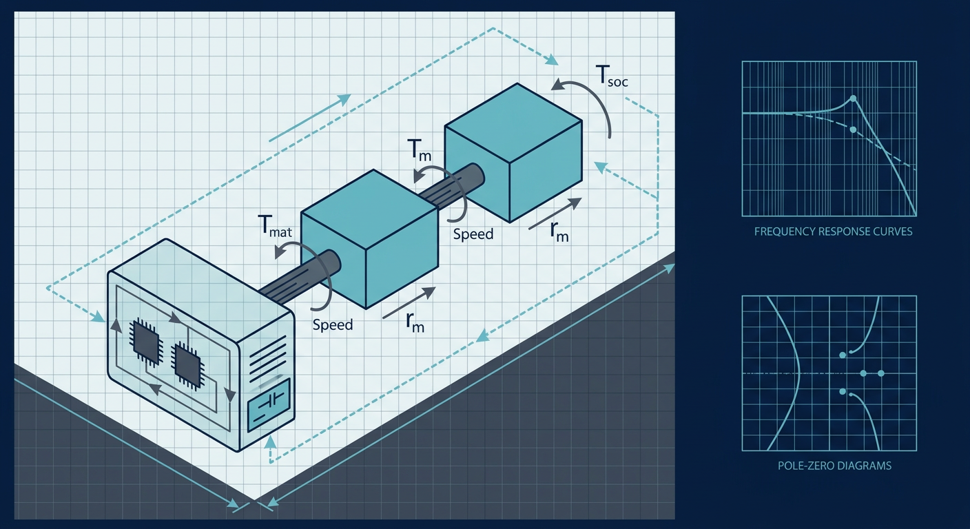
Electric vehicle drivetrains are deceptively elastic. When an inverter demands 350 Nm of regenerative braking torque in under 40 milliseconds, it does not act against a rigid mass. It torques a lightweight permanent magnet rotor coupled through an intermediate gearbox, differential, and slender steel half-shafts to the vehicle inertia. That compliant mechanical chain creates a lightly damped two-mass oscillator with a dominant resonant frequency sitting between 10 Hz and 45 Hz.
Recent drivetrain dynamics studies published in SAE and IEEE transactions highlight a persistent calibration headache. When drivers abruptly lift off the accelerator pedal or when traction control commands rapid torque cuts, this low-frequency resonance gets excited. The driver feels a harsh longitudinal shuffle, often termed tip-out clunk or drivetrain shudder. The traditional calibration fix, slapping a first-order or second-order low-pass filter on the driver torque request, solves the oscillation by destroying transient responsiveness. It turns an agile electric motor into something that feels as sluggish as a turbocharged engine with turbo lag.
Calibration teams and mechatronics engineers do not need to sacrifice throttle response to eliminate shudder. By treating the inverter as a high-bandwidth active actuator, we can inject an active damping torque component that extracts mechanical energy from the half-shafts at the exact resonant frequency. Doing this reliably requires rigorous plant identification using swept-sine chirps and precise pole-zero placement in the discrete domain.
The Mechanical Plant: Two-Mass Resonance and Anti-Resonance
To control half-shaft twist, you must first understand the open-loop transfer function seen by the inverter current controller. A simplified lumped-parameter model treats the drivetrain as two rotating inertias connected by a torsional spring and damper:
- Motor rotor and primary reduction gear inertia ($J_m$), with angular position $\theta_m$ and angular velocity $\omega_m$.
- Equivalent vehicle and wheel inertia reflected to the motor side ($J_L$), with angular position $\theta_L$ and angular velocity $\omega_L$.
- Drive shaft equivalent torsional stiffness ($K_s$) and internal material damping ($C_s$).
The equations of motion governing this system are:
$$J_m \ddot{\theta}_m + C_s (\dot{\theta}_m - \dot{\theta}_L) + K_s (\theta_m - \theta_L) = T_m$$
$$J_L \ddot{\theta}_L - C_s (\dot{\theta}_m - \dot{\theta}_L) - K_s (\theta_m - \theta_L) = -T_L$$
Here, $T_m$ is the electromagnetic torque generated by the stator, and $T_L$ represents external load torque from rolling resistance, aerodynamics, and road gradient.
Taking the Laplace transform and solving for the transfer function from motor torque $T_m(s)$ to motor speed $\omega_m(s)$ (assuming zero external load disturbance $T_L = 0$) yields:
$$G_{vm}(s) = \frac{\omega_m(s)}{T_m(s)} = \frac{1}{(J_m + J_L)s} \cdot \frac{J_L s^2 + C_s s + K_s}{\frac{J_m J_L}{J_m + J_L} s^2 + C_s s + K_s}$$
This transfer function reveals the core structural challenge of electric powertrains. The system contains an integrator corresponding to the total lumped inertia $(J_m + J_L)$, a complex zero pair (anti-resonance), and a complex pole pair (resonance).
The anti-resonance frequency $\omega_z$ occurs at:
$$\omega_z = \sqrt{\frac{K_s}{J_L}}$$
The resonant frequency $\omega_p$ occurs at:
$$\omega_p = \sqrt{K_s \left( \frac{1}{J_m} + \frac{1}{J_L} \right)} = \sqrt{\frac{K_s (J_m + J_L)}{J_m J_L}}$$
Because $J_L$ (the vehicle inertia reflected through the final drive ratio squared) is typically 5 to 20 times larger than the rotor inertia $J_m$, the anti-resonance zero frequency $\omega_z$ is significantly lower than the resonance pole frequency $\omega_p$.
On a Bode plot, the magnitude curve drops sharply at $\omega_z$ where the half-shaft acts as a vibration absorber, followed immediately by a sharp resonant peak at $\omega_p$. Crucially, the phase drops through 180 degrees between $\omega_z$ and $\omega_p$. If a baseline speed or torque controller has open-loop bandwidth anywhere near this region, this abrupt phase cliff destroys the phase margin, causing sustained limit cycles or severe ringing during torque transients.
Why Calibration Filters Fall Short
In standard automotive calibration workflows, calibration engineers frequently attempt to suppress tip-in/tip-out oscillations using static lookup tables and output rate-limiters on the accelerator pedal map. The common fallback is an input filter applied to the reference torque $T_{ref}^*$:
$$T_{filtered}(s) = \frac{\omega_c}{s + \omega_c} T_{ref}^*(s)$$
If the mechanical resonance sits at 18 Hz, the corner frequency $\omega_c$ must be pulled down to 4 Hz or 5 Hz to achieve 15 dB of attenuation at resonance.
This brute-force approach introduces two severe engineering penalties:
- Transient Delay: A 5 Hz low-pass filter adds over 30 milliseconds of group delay to the driver torque request. During emergency regen braking or automated collision avoidance interventions, this delay directly lengthens the vehicle stopping distance.
- No Disturbance Rejection: Low-pass filtering the command input does zero work against external torque disturbances. When the vehicle drives over a pothole, manhole cover, or ice patch, the sudden torque step on the wheel side excites the resonance mode directly. An input filter cannot damp an oscillation injected at the plant output.
True active damping does not smooth out the driver command. Instead, it extracts the oscillatory velocity component from high-resolution motor resolver measurements and injects a dynamic compensating torque back into the inverter current loop.
Swept-Sine Chirp Plant Identification
Before designing an active damping filter, you must pinpoint $\omega_z$, $\omega_p$, and the damping ratio $\zeta$ of the physical drivetrain. Theoretical finite element models are rarely accurate enough because tire carcass compliance, rubber suspension bushings, and CV joint flexibilities alter the effective stiffness $K_s$ under load.
The most dependable method to extract the true frequency response is an in-vehicle or dyno-based swept-sine chirp test.
Excitation Signal Design
To prevent the inverter from saturating or breaking vehicle traction, inject a band-limited logarithmic chirp torque perturbation $T_{chirp}(t)$ directly into the $q$-axis current controller reference while the vehicle operates at a steady baseline speed:
$$T_{ref}(t) = T_{bias} + A(t) \sin \left( 2\pi f_0 \left( \frac{f_1}{f_0} \right)^{t/T_{dur}} t \right)$$
Key parameters for a typical C-segment passenger EV:
- Baseline torque $T_{bias}$: 40 Nm (keeps drivetrain backlash loaded in one direction).
- Chirp amplitude $A(t)$: 15 Nm peak.
- Frequency range: $f_0 = 1\text{ Hz}$ to $f_1 = 80\text{ Hz}$.
- Sweep duration $T_{dur}$: 30 seconds.
Data acquisition must capture motor angular velocity $\omega_m$ directly from the motor resolver interface at the inverter switching frequency (typically 8 kHz or 10 kHz) or sampled synchronously at the speed-loop rate (typically 1 kHz).
Coherence and Spectral Estimation
Compute the Empirical Transfer Function Estimate (ETFE) using Welch's averaged periodogram method. Window the recorded torque command $T_m(t)$ and resolver speed output $\omega_m(t)$ with a 50% overlapping Hanning window:
$$\hat{G}{vm}(j\omega) = \frac{\hat{P}{T\omega}(j\omega)}{\hat{P}_{TT}(j\omega)}$$
Always check the magnitude squared coherence $\gamma^2(\omega)$ before fitting transfer function coefficients:
$$\gamma^2(\omega) = \frac{|\hat{P}{T\omega}(j\omega)|^2}{\hat{P}{TT}(j\omega) \hat{P}_{\omega\omega}(j\omega)}$$
If $\gamma^2(\omega) < 0.85$ around the resonant band, the identification is invalid. Poor coherence in this test typically indicates that the torque excitation was too low, allowing gear backlash to chatter across the mechanical deadband, or that road surface roughness dominated the resolver signal.
+--------------------------------------------------------------------------------+
| ILLUSTRATIVE COMPOSITE: IDENTIFICATION & ACTIVE DAMPING BENCHMARK              |
| Baseline 150 kW Interior Permanent Magnet Synchronous Motor (IPMSM) Powertrain |
| Plant parameters: J_m = 0.042 kg*m^2, J_L = 0.68 kg*m^2 (motor side),           |
| Half-shaft K_s = 2,450 Nm/rad. Controller sampled at Ts = 100 microseconds.    |
+---------------------------------------+-------------+-------------+------------+
| Performance Metric                    | Unmitigated | 5 Hz LP     | Active     |
|                                       | Open Loop   | Filter      | Damping BP |
+---------------------------------------+-------------+-------------+------------+
| Measured Resonance Peak f_p (Hz)      | 23.4 Hz     | 23.4 Hz     | Suppressed |
| Torque Step 0-90% Rise Time (ms)      | 12.0 ms     | 68.5 ms     | 14.5 ms    |
| Half-Shaft Torque Overshoot (%)       | 84.2%       | 6.1%        | 7.8%       |
| Settling Time to +/-5% Band (ms)      | 240.0 ms    | 92.0 ms     | 28.0 ms    |
| Peak Sensitivity Margin M_s           | 3.82        | 1.15        | 1.34       |
| Phase Margin at Gain Crossover (deg)  | 18.2 deg    | 52.0 deg    | 64.5 deg   |
+---------------------------------------+-------------+-------------+------------+
Active Damping Architecture: Bandpass State Feedback
Once $\omega_p$ and the plant structure are identified, the inverter software can implement an active damping torque loop. The goal is to generate a damping torque $T_{damp}$ that acts as a virtual damper in parallel with the half-shafts.
The most robust industrial structure uses a bandpass filter applied to the motor velocity. The total motor torque command $T_m^*$ sent to the inner current loop becomes:
$$T_m^(s) = T_{driver}^(s) - H_{ad}(s) \omega_m(s)$$
Where $H_{ad}(s)$ is a second-order bandpass filter centered directly on the identified resonant frequency $\omega_p$:
$$H_{ad}(s) = K_d \frac{2 \zeta_f \omega_p s}{s^2 + 2 \zeta_f \omega_p s + \omega_p^2}$$
In this formulation:
- $K_d$ is the active damping gain (units of $\text{Nm}/(\text{rad}/\text{s})$).
- $\omega_p$ is the identified mechanical resonant frequency in rad/s.
- $\zeta_f$ is the filter damping ratio, which controls the width of the active damping frequency passband.
The Pole-Zero Placement Mechanism
Why does a bandpass filter work so effectively here?
At DC and low frequencies ($s \to 0$), $H_{ad}(s) \approx 0$. This ensures the active damping loop does not fight steady-state acceleration, vehicle hill-climbing, or steady regenerative braking. The vehicle can cruise or hold torque without steady-state tracking error.
At high frequencies ($s \to \infty$), $H_{ad}(s) \approx 0$. This ensures high-frequency resolver noise, inverter switching ripple, and electromagnetic cogging harmonics are not amplified into the motor current loop.
At the resonant frequency ($s = j\omega_p$), the transfer function evaluates to:
$$H_{ad}(j\omega_p) = K_d$$
The filter output is purely real and in phase with the motor speed oscillation $\omega_m(j\omega_p)$. Multiplying this in-phase speed by $K_d$ creates an electronic damper torque directly opposing the torsional velocity oscillation. This shifts the lightly damped complex poles of the closed-loop system deep into the left half of the s-plane, artificially boosting the equivalent mechanical damping ratio from $\zeta \approx 0.03$ up to $\zeta_{eff} \approx 0.40$.
Discrete-Time Implementation via Bilinear Transform
Running active damping inside a microcontroller or digital signal processor requires converting $H_{ad}(s)$ into a discrete biquad filter. A direct Euler approximation will distort the resonant peak and introduce phase errors that can destabilize the loop.
Use the Tustin bilinear transform with frequency pre-warping to preserve the exact center frequency $\omega_p$ at a given sample period $T_s$:
$$\omega_w = \frac{2}{T_s} \tan \left( \frac{\omega_p T_s}{2} \right)$$
Substitute $s = \frac{2}{T_s} \frac{1 - z^{-1}}{1 + z^{-1}}$ into the continuous pre-warped filter:
$$H_{ad}(z) = \frac{b_0 + b_1 z^{-1} + b_2 z^{-2}}{a_0 + a_1 z^{-1} + a_2 z^{-2}}$$
Let $Q = 2 \zeta_f \omega_w$ and $K_{pre} = \frac{2}{T_s}$. The algebraic coefficients evaluate to:
$$a_0 = K_{pre}^2 + Q K_{pre} + \omega_w^2$$ $$a_1 = 2(\omega_w^2 - K_{pre}^2)$$ $$a_2 = K_{pre}^2 - Q K_{pre} + \omega_w^2$$ $$b_0 = K_d Q K_{pre}$$ $$b_1 = 0$$ $$b_2 = -K_d Q K_{pre}$$
Normalize by dividing all coefficients by $a_0$ to yield standard Direct Form II Transposed difference equations executed on each speed-loop interrupt:
/* Discrete Direct Form II Transposed Biquad Implementation */
typedef struct {
    float b0, b1, b2;
    float a1, a2;
    float w1, w2;
} BiquadFilter;

float ActiveDamping_Update(BiquadFilter *f, float omega_motor_rads) {
    /* Compute filtered damping torque output */
    float y = (f->b0 * omega_motor_rads) + f->w1;

    /* Update internal delay states */
    f->w1 = (f->b1 * omega_motor_rads) - (f->a1 * y) + f->w2;
    f->w2 = (f->b2 * omega_motor_rads) - (f->a2 * y);

    return y; /* Output torque to subtract from driver request */
}
Nonlinearities: Handling Gearbox Backlash
Linear active damping assumes continuous mechanical engagement between the rotor pinion and the ring gear. In reality, every automotive reduction gearbox contains a mechanical clearance deadband, typically $0.15^\circ$ to $0.4^\circ$ of lash.
During a fast transition from drive torque (+200 Nm) to regenerative braking (-200 Nm), the drivetrain crosses through zero torque. While passing through the deadband, the rotor disengages from the wheel inertia entirely. For a few milliseconds, the motor rotor accelerates freely as a single mass with zero effective load ($J_L = 0$).
If the active damping filter continues to run at full gain during this zero-crossing interval, it detects the rapid acceleration across the lash gap as an oscillation. The filter responds by firing a sharp counter-torque, causing the gear teeth to slam into the opposite face with high impact velocity. This manifests as a loud metallic lash clunk.
To prevent lash clunk during regen transitions, implement a nonlinear gain-scheduling supervisor:
- Torque Zero-Crossing Detector: Monitor the requested torque $T_{driver}^$. When $|T_{driver}^| < T_{lash_thresh}$ (typically 10 to 15 Nm), scale down the active damping gain $K_d$ smoothly using a cubic spline transition.
- Backlash State Estimator: Implement a kinematic state observer that tracks the relative angle $\theta_d = \theta_m/N - \theta_L$. When $\theta_d$ is inside the known deadband $[-\alpha_{lash}, +\alpha_{lash}]$, disable active damping and switch the inverter to an open-loop torque slew-rate limiter (e.g., maximum $1.5\text{ Nm}/\text{ms}$) until mechanical contact is re-established.
- Phase-Safe Re-engagement: Once contact on the reverse gear flank is detected via current and speed correlation, ramp $K_d$ back to nominal within 10 milliseconds.
Practical Calibration and Validation Checklist
When bringing up active damping algorithms on a dyno or vehicle prototype, follow this structured execution sequence:
- Lock In Resolver Resolution: Ensure your resolver-to-digital converter (RDC) tracking loop bandwidth is at least $500\text{ Hz}$. Low RDC tracking bandwidth adds artificial phase delay into $\omega_m$, destabilizing the damping loop.
- Execute Swept-Sine Baseline: Inject chirps from 1 Hz to 80 Hz under positive torque load. Confirm that the coherence metric $\gamma^2(f) > 0.85$ across the 10 Hz to 45 Hz band.
- Extract Resonance Poles: Record the exact frequency of the resonance peak $\omega_p$. Note whether shifts occur across different vehicle loading states (e.g., unladen vs. gross vehicle weight).
- Tune Filter Q-Factor: Set $\zeta_f$ between $0.35$ and $0.5$. A filter with a Q-factor that is too narrow will miss the resonance if tire wear or temperature changes half-shaft compliance; a filter that is too wide will degrade phase margin outside the resonant band.
- Sweep Damping Gain $K_d$: Increment $K_d$ gradually from zero while performing 100% tip-in and tip-out torque steps. Measure settling time and peak overshoot on a wireless half-shaft torque telemetry collar.
- Validate Sensitivity Peak ($M_s$): Measure the closed-loop sensitivity function $S(j\omega) = \frac{1}{1 + G(j\omega) H(j\omega)}$. Ensure the peak sensitivity $M_s = \max_\omega |S(j\omega)|$ remains strictly below $1.4$ ($3\text{ dB}$) across all operating speeds to guarantee robust stability.
- Verify Thermal and Inverter Headroom: Check that the added dynamic damping current does not push the inverter power modules (IGBT/SiC MOSFETs) into instantaneous overcurrent protection during rapid tip-out cycles.
What This Means for LabCD
Designing active damping controllers that hold up under real mechanical backlash, variable tire grip, and hard regenerative braking requires moving beyond trial-and-error PID heuristics. LabCD (labcd.ai) enables controls and mechatronics teams to load swept-sine empirical frequency responses, identify parametric multi-mass models with bounded uncertainty, and synthesize discrete active damping filters with proven sensitivity and phase margins. By generating deterministic, production-ready C code directly from identified plant models, LabCD provides the receipts engineering teams need before flashing inverter firmware.
Summary Direct Answer
How do you eliminate EV drivetrain shudder during regenerative braking without making throttle response sluggish? Do not use aggressive low-pass filtering on the driver torque demand. Instead, identify the half-shaft two-mass resonant frequency using swept-sine chirp excitation, and implement an inverter-based active damping feedback loop using a discrete second-order bandpass filter. The bandpass filter extracts the velocity oscillation at the resonant peak and injects an opposing damping torque directly into the motor current loop, suppressing half-shaft oscillation within one cycle while preserving full transient torque response.
Sources
- SAE Technical Paper 2023-01-0538: Torsional Vibration Analysis and Control in Electric Powertrains: https://www.sae.org/publications/technical-papers/content/2023-01-0538/
- IEEE Transactions on Power Electronics (Document 9760124): Active Torsional Vibration Suppression for Electric Vehicle Drivetrains: https://ieeexplore.ieee.org/document/9760124
- ScienceDirect / Control Engineering Practice: Modelling and Active Damping of Torsional Vibration in Powertrain Systems: https://www.sciencedirect.com/science/article/abs/pii/S0967066120302045
- MDPI Machines: Active Control of Torsional Vibration during Mode Switching of Electric Powertrains: https://www.mdpi.com/2075-1702/10/8/647
- SAGE Journals: Vibration and Dynamics Analysis of Electric Vehicle Drivetrains: https://journals.sagepub.com/doi/10.1177/1461348420979204