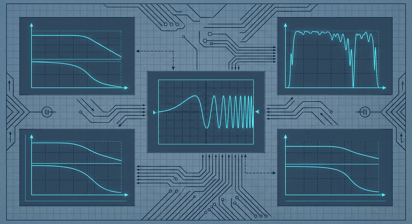
Control engineers frequently inherit rigid-body CAD assemblies, run a quick step test to calculate dominant time constants, tune a feedback loop in simulation, and watch the real hardware oscillate the moment loop gain is raised. Step inputs put most of their spectral energy at direct current. They excite low-frequency rigid dynamics while starving the high-frequency modes where structural compliance, backlash, and actuator current limits live. When the physical machine operates, unmodeled phase lag at higher frequencies erodes phase margin, turning a supposedly robust controller into a physical vibrator.
Recent discussions across the control theory community and updated guidance in aerospace flight-test identification protocols reinforce an old lesson: you cannot control what you have not excited. If your identification data lacks signal energy across the crossover frequency, your mathematical plant model is an extrapolation. Extracting the real input-output behavior of a physical mechanism requires deliberate frequency-domain input design. By structuring swept-sine, chirp, and multisine signals to deliver uniform power across a target bandwidth, mechatronics teams can extract clean non-parametric frequency response functions, verify data validity using spectral coherence, and fit bounded uncertainty models suitable for robust synthesis.
Why Step Tests and CAD Inertias Lie
A mechanical CAD assembly calculates theoretical mass properties with geometric perfection. It assumes infinite structural stiffness, perfectly rigid couplings, zero bearing play, and linear magnetic flux in the motors. Real mechatronics hardware violates every one of these assumptions. Fasteners have micro-slip, timing belts act as non-linear springs, harmonic drives exhibit gear transmission error, and power electronics introduce phase delay through pulse-width modulation filters and analog-to-digital conversions.
When an engineer tries to capture these dynamics using a simple step response, the input power spectral density drops off at twenty decibels per decade. The signal dumps almost all its energy into driving the plant across its large-displacement low-frequency range. By the time the energy reaches the first structural anti-resonance or torsional mode, the signal-to-noise ratio is completely degraded. What looks like minor sensor ripple on an oscilloscope is often the decaying signature of a resonance mode that will destabilize a high-bandwidth velocity or position loop.
Fitting a transfer function to a noisy step response forces the identification algorithm to minimize time-domain squared errors. The optimizer prioritizes the large-amplitude low-frequency trajectory and ignores high-frequency residuals. The resulting model fits the step test visually, but its phase prediction at the desired crossover frequency can be wrong by forty-five degrees or more. Closing the loop with aggressive proportional or integral gains based on that model is an immediate recipe for limit cycles or mechanical damage.
Step Input Energy Spectrum:
|Power (dB)
|***
|   ****
|       ****
|           **** (-20 dB/decade roll-off)
|               **** (High-frequency resonance buried in noise floor)
+-----------------------------------> Frequency (Hz)

Broadband Excitation Energy Spectrum:
|Power (dB)
|*********************************** (Uniform spectral power density)
|                                  *
|                                  * (Resonance clearly revealed)
+-----------------------------------> Frequency (Hz)
The Anatomy of Identification Signals
Frequency-domain system identification relies on persistent excitation across the entire frequency range where the controller must remain stable. This includes not just the operating bandwidth, but at least one to two octaves beyond the target gain crossover frequency. Three primary signal classes dominate practical mechatronics and flight-test identification.
Linear and Logarithmic Swept-Sines (Chirps)
A chirp signal sweeps a sinusoidal tone continuously from a starting frequency $f_1$ to an end frequency $f_2$ over a duration $T$. The instantaneous frequency can vary linearly or logarithmically.
Linear sweeps distribute equal energy per Hertz across the spectrum. They work well for narrow-band plant investigation where resonant frequencies are already approximately known. The instantaneous phase $\phi(t)$ for a linear chirp is defined as:
$$\phi(t) = 2\pi \left( f_1 t + \frac{f_2 - f_1}{2T} t^2 \right)$$
Logarithmic sweeps distribute equal energy per octave or decade, spending more time at low frequencies and sweeping rapidly through high frequencies. Because control engineers evaluate stability margins on logarithmic frequency scales, logarithmic chirps provide consistent signal-to-noise ratios across every decade of interest. The instantaneous phase for a logarithmic chirp is defined as:
$$\phi(t) = 2\pi f_1 \left( \frac{k^t - 1}{\ln(k)} \right), \quad \text{where } k = \left(\frac{f_2}{f_1}\right)^{1/T}$$
When executing chirps on physical actuators, you must ramp the amplitude smoothly at the start and end of the sweep using a Tukey or Hann window. Hard starts inject broadband transient spikes that can trip overcurrent limits on motor drives or saturate mechanical stops.
Pseudo-Random Binary Sequences (PRBS)
A Pseudo-Random Binary Sequence is a deterministic, periodic signal that switches between two discrete levels, $+A$ and $-A$, based on a linear feedback shift register. A PRBS generated by an $n$-bit register has a sequence length of $N = 2^n - 1$ clock periods $\Delta t$.
PRBS signals approximate white noise while maintaining a perfectly bounded amplitude. The auto-correlation of a full PRBS period is close to a Dirac delta function, creating a nearly flat power spectrum up to a cutoff frequency proportional to $1/\Delta t$. The spectral envelope follows a squared sinc function:
$$S_{xx}(f) \propto \left( \frac{\sin(\pi f \Delta t)}{\pi f \Delta t} \right)^2$$
To ensure flat power across your identification bandwidth $f_{max}$, choose the clock period such that the bandwidth sits well inside the first main lobe, typically setting $\Delta t \le 1 / (2.5 f_{max})$. PRBS signals are easy to implement on embedded microcontrollers because they require only bit-shift operations and sign changes. However, their sharp square edges will excite unmodeled dynamics far above the Nyquist frequency, causing actuator slew-rate saturation unless filtered through a low-pass digital filter prior to drive execution.
Optimized Multisines and Crest Factor Minimization
A multisine is a sum of harmonically related sinusoids with user-defined amplitudes and phases:
$$u(t) = \sum_{k=1}^{M} A_k \cos(2\pi f_k t + \phi_k)$$
If all phases $\phi_k$ are set to zero, the sinusoids align constructively at $t=0$, creating a massive peak in the time domain while delivering low root-mean-square (RMS) power throughout the rest of the period. This results in a high Crest Factor ($CF$), defined as the ratio of peak absolute value to RMS value:
$$CF(u) = \frac{\max_{t} |u(t)|}{u_{\text{RMS}}}$$
A high crest factor is disastrous for plant identification. The actuator hits its current, torque, or displacement limits at the peak, while the rest of the signal barely rises above the sensor noise floor. To maximize energy injection without saturating the plant, engineers optimize the phase vector $\phi_k$ using algorithms like the Schroeder phase selection:
$$\phi_k = \phi_1 - \frac{\pi k(k - 1)}{M}$$
Schroeder phasing spreads the individual sine peaks evenly throughout the time period, dropping the Crest Factor from over $5.0$ down to below $1.8$. This allows an engineer to inject double the RMS power into the plant without exceeding physical voltage or travel bounds.
Signal Type Comparison for Bench Identification:

+-------------------+---------------+------------------+-----------------------+
| Signal Type       | Crest Factor  | Frequency Target | Primary Limitation    |
+-------------------+---------------+------------------+-----------------------+
| Pure Step         | High (1.0+)   | DC only          | High-frequency blind  |
| Linear Chirp      | ~1.414        | Uniform (Hz)     | Slow over wide sweeps |
| Log Chirp         | ~1.414        | Uniform (Octaves)| Transient settling    |
| PRBS              | 1.000         | Broad band       | Slew-rate saturation  |
| Multisine (Schr.) | 1.40 - 1.80   | Discrete grids   | Setup complexity      |
+-------------------+---------------+------------------+-----------------------+
Spectral Coherence: The Truth Filter
Once an input signal $u(t)$ is applied and the output response $y(t)$ is recorded, the raw data must not be fed straight into a parameter estimator. You must first compute the non-parametric empirical transfer function estimate and evaluate its spectral coherence $\gamma_{xy}^2(f)$.
Using Welch's averaged periodogram method, the data is split into overlapping windowed segments to estimate the input auto-spectral density $\hat{S}{uu}(f)$, the output auto-spectral density $\hat{S}{yy}(f)$, and the cross-spectral density $\hat{S}_{uy}(f)$. The non-parametric frequency response function $\hat{G}(j\omega)$ is calculated via the $H_1$ estimator, which minimizes the effect of output measurement noise:
$$\hat{G}(j\omega) = \frac{\hat{S}{uy}(f)}{\hat{S}{uu}(f)}$$
The magnitude-squared coherence function is defined as:
$$\gamma_{uy}^2(f) = \frac{|\hat{S}{uy}(f)|^2}{\hat{S}{uu}(f) \hat{S}_{yy}(f)}$$
Coherence is a scalar metric bounded strictly between $0.0$ and $1.0$ at each frequency point. In an ideal, perfectly linear system with noiseless sensors, coherence equals exactly $1.0$ across the entire spectrum. In physical testing, a drop in coherence indicates one of three phenomena:
- Low Signal-to-Noise Ratio: The input energy at that frequency is too weak relative to sensor noise. The estimated transfer function is dominated by random drift.
- Non-linear Distortion: The plant contains non-linear dynamics, such as static friction, backlash, or amplifier saturation, that generate output frequencies not present in the input.
- Unmeasured Disturbances: External forces, thermal expansion, or mechanical vibrations from adjacent equipment are corrupting the output channels.
Typical Coherence Interpretation:

Coherence (gamma^2)
1.0 +-----------------------------------------------
    | Valid Data Zone: Trust model for tuning
0.8 + - - - - - - - - - - - - - - - - - - - - - - - -
    | Caution Zone: Average more runs or boost power
0.6 + - - - - - - - - - - - - - - - - - - - - - - - -
    | Invalid Data Zone: Pure noise or non-linearity
0.0 +-----------------------------------------------
    0 Hz                                      f_max
A common failure in controls development is fitting high-order transfer functions to frequency bands where coherence drops below $0.7$. An identification optimizer will bend poles and zeros to match random measurement noise in low-coherence regions, creating phantom resonances. The rule for plant validation is simple: strip out or de-weight all frequency points where coherence is inadequate before fitting parametric transfer functions.
Establishing Bounded Uncertainty for Synthesis
A single nominal transfer function $G_0(s)$ is never sufficient for high-performance controller synthesis. Real physical plants change their behavior with temperature, payload variations, and operating points. A complete frequency-domain identification protocol requires measuring the plant across multiple operating conditions and calculating an upper bound on dynamic uncertainty.
Let the set of identified plant frequency responses across multiple sweeps and operating points be denoted by $G_k(j\omega)$ for $k = 1, \dots, N$. The nominal model $G_0(s)$ is fitted to the average response. The relative multiplicative dynamic uncertainty $l_m(\omega)$ is calculated as the maximum deviation at each frequency:
$$l_m(\omega) = \max_{k} \left| \frac{G_k(j\omega) - G_0(j\omega)}{G_0(j\omega)} \right|$$
Control engineers then fit a stable, minimum-phase rational weighting filter $W_m(s)$ such that its magnitude envelopes the uncertainty across all frequencies:
$$|W_m(j\omega)| \ge l_m(\omega), \quad \forall \omega$$
Multiplicative Uncertainty Envelope:
|Magnitude (dB)
|                      /-------- Bounds: |Wm(jw)|
|          ...*......./   ***
|       .*.   *  .***    *   *  <- Experimental Data: lm(w)
|    ..*       **
|...*
+-----------------------------------> Frequency (rad/s)
This weighting filter forms the mathematical receipt for robust synthesis. According to the small gain theorem, a feedback controller $K(s)$ tuned for the nominal plant $G_0(s)$ will remain robustly stable for all perturbed physical plants within the family if and only if the complementary sensitivity function $T(s) = \frac{G_0(s)K(s)}{1 + G_0(s)K(s)}$ satisfies:
$$| W_m(s) T(s) |_{\infty} < 1$$
Designing the controller against this explicit bound eliminates the guess-and-check tuning cycle. If the synthesized loop respects this inequality, the system is mathematically guaranteed not to oscillate when deployed across hardware units with normal manufacturing tolerances.
Comparative Receipts on Actuator Identification
To demonstrate the practical difference between input signals, consider an illustrative composite testbench consisting of a brushless motor coupled to a flexible compliance fixture with a torsional load. The setup represents a common industrial positioning stage where high-frequency resonance limits closed-loop gains. In this composite dataset, five standard excitation schemes were run under identical physical operating conditions.
Illustrative Composite: Identification Signal Performance
Actuator: 200W PMSM with 20-bit optical encoder and flexible shaft load
Acquisition: 10 kHz sample rate, 50 Hz target bandwidth, 0 to 500 Hz sweep range
Tooling: Frequency-domain Welch estimator with 50% overlap Hann windowing

+------------------+-------------+---------------+-------------------+-------------------+
| Input Signal     | Crest       | Mean SNR      | Coherence >= 0.9  | Estimated First   |
| Type             | Factor (CF) | (0 - 500 Hz)  | Bandwidth (Hz)    | Resonance (Hz)    |
+------------------+-------------+---------------+-------------------+-------------------+
| Step Pulse       | 3.82        | 11.4 dB       | 0 - 32 Hz         | Undetected (NaN)  |
| White Noise      | 3.45        | 16.8 dB       | 0 - 110 Hz        | 184 Hz (+/-18 Hz) |
| Linear Chirp     | 1.41        | 28.2 dB       | 0 - 410 Hz        | 191.2 Hz (+/-1.2) |
| Log Chirp        | 1.42        | 31.5 dB       | 0 - 465 Hz        | 191.8 Hz (+/-0.8) |
| Opt. Multisine   | 1.68        | 33.1 dB       | 0 - 490 Hz        | 192.1 Hz (+/-0.4) |
+------------------+-------------+---------------+-------------------+-------------------+
In this composite test, the step pulse failed completely to resolve the compliance resonance at 192 Hz because its power had dropped into the encoder quantization noise floor. An engineer relying on the step test would have concluded the actuator behaved like a pure rigid inertia, leading to a PID tuning with a phase margin deficit of thirty degrees at the resonant frequency.
Unfiltered white noise pushed excessive instantaneous peak torques, causing minor current clipping that generated non-linear harmonics and degraded coherence above 110 Hz. The Schroeder-optimized multisine and the logarithmic chirp delivered clean coherence across nearly the entire 500 Hz analysis window, locating the 192.1 Hz resonant pole and its accompanying zero with less than one Hertz of estimation variance.
Practical Protocol for Frequency-Domain Testing
Before running any excitation sequence on physical hardware, follow this operational checklist to protect the mechanism and obtain defensible identification data:
- Establish Quiescent Operating Points: Always inject the identification signal around a steady-state equilibrium operating point. If testing an axis subject to gravity, maintain the bias holding torque before superimposing the dynamic perturbation.
- Verify Linear Amplitude Limits: Run a sequence of three sweeps at 25%, 50%, and 100% of your planned test amplitude. Superimpose the estimated transfer functions. If the resonant peaks shift significantly in frequency or drop drastically in gain as amplitude increases, the system is exhibiting non-linear saturation or Coulomb friction. Lower the excitation amplitude until the frequency response scales linearly.
- Enforce Integral Periodicity: When using multisine signals, ensure that the total acquisition time is an exact integer multiple of the fundamental period of the lowest frequency component. This prevents spectral leakage in the Discrete Fourier Transform and avoids the need for heavy windowing corrections.
- Check Actuator Slew Rates: Compute the time derivative of your designed input signal. Ensure that the required voltage, current, or valve-spool rate does not exceed the continuous slew-rate capability of your drive electronics.
- Compute and Save Coherence Masks: Automatically drop data points where coherence is below 0.8 prior to fitting transfer functions. Save the coherence plot directly alongside the Bode diagram as the formal validation receipt for design reviews.
Identification Execution Flow:

[ Define Frequency Range: f_min to f_max ]
                   |
                   v
[ Generate Signal: Log Chirp or Schroeder Multisine ]
                   |
                   v
[ Apply Tukey Window to Prevent Transient Spikes ]
                   |
                   v
[ Inject at Actuator Drive & Record Output at Sensor ]
                   |
                   v
[ Compute Welch Cross-Spectra: S_uu, S_yy, S_uy ]
                   |
                   v
[ Evaluate Coherence: gamma^2(f) >= 0.8? ]
        |                         |
      (Yes)                      (No)
        v                         v
[ Fit Parametric Transfer   [ Flag Low SNR / Non-Linearity;
  Function G_0(s) ]           Adjust Amplitude or Re-test ]
        |
        v
[ Extract Uncertainty Filter W_m(s) for Synthesis ]
What this means for LabCD
Control design platforms cannot assume that theoretical CAD models represent physical reality. LabCD incorporates frequency-domain identification workflows directly into the controller tuning pipeline. By integrating automated multisine excitation generation, real-time coherence calculation, and non-parametric spectral fitting, the environment lets engineers move from physical bench measurements to robustly tuned PID and MPC controllers without leaving the validation workspace. Plant uncertainty bounds are calculated automatically from experimental sweeps, ensuring that every synthesized controller comes backed by formal gain and phase margin receipts on the real hardware.
The Path to Repeatable Closed-Loop Performance
Moving a mechatronics project from a shaky prototype to a production-ready system requires abandoning trial-and-error bench tuning. If your tuning workflow relies on manually dragging sliders until a step response looks smooth on a bench scope, you are accumulating technical debt that will surface as field failures, mechanical wear, and acoustic noise.
Frequency-domain system identification replaces intuition with verifiable dynamic data. By designing input signals that respect actuator limits while pumping uniform power across the critical crossover frequencies, you strip out the guesswork. You identify the structural compliance, measure the real sensor delays, and define the exact uncertainty envelopes that bound your system. When you present a controller design at a technical review, you do not show that the loop feels calm. You show the coherence spectrum, the identified plant model, and the robust stability proofs that guarantee it will stay calm.
Sources
- System Identification Methods for Aircraft Flight Control Development: https://rosap.ntl.bts.gov/view/dot/12583
- Excitation Signals for Identification of Dynamic Systems: https://sciengineer.com/excitation-signals-for-identification-of-dynamic-systems/
- Pintelon, R. and Schoukens, J., Frequency Domain System Identification: https://link.springer.com/rwe/10.1007/978-1-4471-5102-9_108-1
- Optimal Plant Friendly Input Design for System Identification: https://pubs.acs.org/doi/abs/10.1021/ie200472s
- System Identification Overview and Best Practices: https://www.mathworks.com/help/ident/gs/about-system-identification.html
- System Identification in Underactuated Robotics: https://underactuated.mit.edu/sysid.html