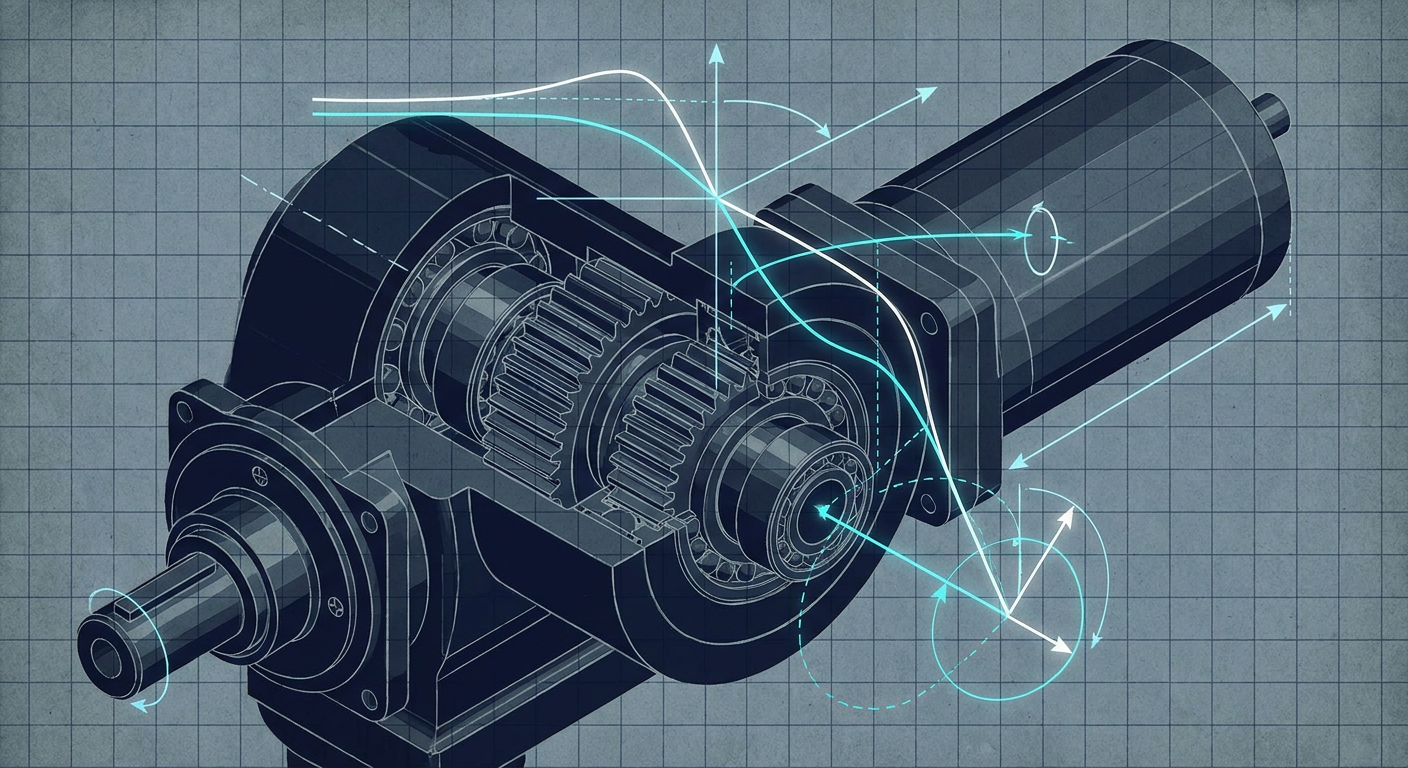
When a tethered biped or robotic manipulator suddenly starts thrashing at twenty hertz, the physical damage happens in seconds. Gear teeth strip inside planetary reducers, cross-roller bearings brinell under rapid load reversals, and inverter bridges pop as motor phase currents surge against saturated limits. Recent viral footage from trade shows, including the widely shared incident at the Beijing World Robot Conference where an actuated demonstration unit violently lost stability and thrashed against the floor, highlights a reality that every mechatronics lead knows privately: violent instability rarely comes from pure software crashes. It comes from closed-loop control systems crossing the boundary between small-signal linear stability and non-linear limit cycles.
For control engineers, faculty researchers, and robotics R&D teams, runaway oscillation is one of the most expensive failure modes in the field. It burns through hardware budgets, delays academic publications, and destroys confidence during live hardware demonstrations. More critically, it exposes a fundamental flaw in the design workflow: tuning feedback loops against idealized rigid-body simulations rather than identified physical plants with real phase lag, structural resonance, and finite actuator headroom.
Preventing high-frequency instability requires understanding the specific physical and algorithmic mechanisms that turn a seemingly stable feedback loop into a self-sustaining mechanical hammer.
The Anatomy of a High-Frequency Limit Cycle
Linear control theory tells us that a system is stable if its open-loop transfer function $L(s) = C(s)P(s)$ maintains positive gain and phase margins. If the loop gain $|L(j\omega)|$ drops below unity ($0\text{ dB}$) before the phase angle reaches $-180^\circ$, linear perturbations decay exponentially.
In real actuated hardware, linear stability is merely a local condition. Actuators have finite voltage rails, current limits, and slew rates. Sensors introduce quantization and phase delay. Structural components possess flexible modes.
When a disturbance excites an unmodeled high-frequency dynamic, the controller demands rapid corrective torque. If that demand exceeds the inverter current clamp or the motor's back-EMF headroom, the effective gain of the actuator drops. In classical frequency-domain terms, the saturation behaves as a non-linear gain described by a Describing Function $N(A)$, where $A$ is the amplitude of the sinusoidal input to the non-linear element:
$$N(A) = \frac{2}{\pi} \left( \arcsin\left(\frac{u_{\text{max}}}{A}\right) + \frac{u_{\text{max}}}{A} \sqrt{1 - \left(\frac{u_{\text{max}}}{A}\right)^2} \right) \quad \text{for } A > u_{\text{max}}$$
As the oscillation amplitude $A$ grows, the effective gain $N(A)$ decreases. If the Nyquist plot of the linear loop $L(j\omega)$ wraps around or intersects the negative reciprocal of the describing function, $-1/N(A)$, the system locks into an autonomous limit cycle. The hardware does not experience an unbounded exponential explosion. Instead, it locks into a maximum-energy, violent oscillation determined by actuator saturation boundaries, violently shaking until an emergency stop trips or mechanical failure intervenes.
                  +-----------------------------------------+
                  |                                         |
                  v                                         |
[ Reference ] -> (+) -> [ Controller ] -> [ Saturation ] -> [ Flexible Plant ] --+-> [ Output ]
                          C(s)             u_max / slew      P(s) with Res.       |
                                                                                  |
                                 [ Phase-Lagged Filter ] <------------------------+
                                       H(z) / Delay
To eliminate these failures, engineering teams must dissect the four dominant physical and computational root causes that push mechatronic systems across the stability margin.
Four Root Causes of Closed-Loop Runaway
1. The Hidden Phase Penalty of Digital Filtering
In raw actuator data, velocity signals calculated by differentiating raw optical or magnetic encoder counts contain severe quantization noise. High-frequency derivative spikes heat motor coils and saturate inner torque loops. The standard mechatronics fix is straightforward: drop a low-pass filter on the velocity feedback path.
Many teams insert a second-order Butterworth filter or a moving-average FIR filter without recalculating the total open-loop phase budget. Every low-pass filter introduces phase lag well below its cutoff frequency.
A continuous second-order Butterworth filter with cutoff frequency $\omega_c$ introduces a phase shift given by:
$$\phi(\omega) = -\arctan\left( \frac{\sqrt{2} \frac{\omega}{\omega_c}}{1 - \left(\frac{\omega}{\omega_c}\right)^2} \right)$$
At one-third of the cutoff frequency ($\omega = 0.33\omega_c$), the filter already injects roughly $28^\circ$ of phase lag. When implemented on a discrete microcontroller or field-oriented control (FOC) inverter board, additional digital delays accumulate:
- Zero-Order Hold (ZOH) Delay: An average phase lag of $\Delta \phi_{\text{ZOH}} = -\omega T_s / 2$, where $T_s$ is the sampling period.
- Computation and Transport Latency: A delay of one full sample clock between sensor reading and PWM duty cycle update adds another $\Delta \phi_{\text{comp}} = -\omega T_s$.
- Communication Bus Latency: EtherCAT, CAN FD, or SPI frame serialization introduces asynchronous packet jitter and buffering delays.
If the velocity control loop has an intended crossover frequency of $60\text{ Hz}$, but the filter and transport chain contribute $45^\circ$ of unexpected phase drop at that same frequency, a nominal phase margin of $50^\circ$ collapses to $5^\circ$. A minor load disturbance or mechanical backlash immediately sends the joint into sustained resonance.
2. High Sensitivity Peaks and the Waterbed Effect
Control loops tuned purely for fast step-response rise times frequently violate fundamental frequency-domain conservation laws. Bode's sensitivity integral (the waterbed effect) states that for any open-loop stable plant with relative degree greater than one, the integral of the log sensitivity function $S(s) = (1 + L(s))^{-1}$ over all frequencies is zero:
$$\int_{0}^{\infty} \ln |S(j\omega)| , d\omega = 0$$
If a controller aggressively suppresses low-frequency tracking errors (forcing $|S(j\omega)| \ll 1$ below $10\text{ Hz}$), the sensitivity curve must pop above unity ($|S(j\omega)| > 1$) at higher frequencies. The peak of this sensitivity function, denoted as $M_s = \max_\omega |S(j\omega)|$, directly measures loop robustness.
- A well-damped, robust industrial loop maintains $M_s < 1.4$ to $1.6$ (equivalent to gain margin $> 6\text{ dB}$ and phase margin $> 45^\circ$).
- When high proportional and integral gains are dialed in to eliminate joint droop under gravity, $M_s$ often exceeds $2.5$ or $3.0$.
When $M_s = 3.0$, any external disturbance or structural vibration near the peak sensitivity frequency $\omega_{peak}$ is amplified by $300%$ within the loop. The controller actively feeds energy into the plant's mechanical resonances rather than damping them.
3. Unmodeled Drive Compliance and Anti-Resonance
Most robotic joints are modeled as single-mass rigid systems where torque directly produces angular acceleration: $\tau = J \ddot{\theta}$. Real actuators use cycloidal gearboxes, harmonic drives, or planetary gearheads with finite torsional stiffness.
A realistic joint is at least a two-mass system: the motor rotor inertia $J_m$, connected through a torsional spring $K_t$ and internal damping $D_t$ to the link inertia $J_l$. The transfer function from motor torque $\tau_m$ to motor velocity $\omega_m$ reveals a distinct anti-resonance frequency $\omega_{ar}$ followed by a resonance frequency $\omega_r$:
$$\omega_{ar} = \sqrt{\frac{K_t}{J_l}}, \qquad \omega_r = \sqrt{K_t \left( \frac{1}{J_m} + \frac{1}{J_l} \right)}$$
Gain (dB)
  |
  |        /\  <-- Resonant Peak (omega_r)
  |       /  \
  |---\  /    \----------------
  |    \/  <-- Anti-Resonant Notch (omega_ar)
  +-----------------------------> Frequency (rad/s)
If an encoder is mounted on the motor side (collocated sensing), the control loop encounters a deep anti-resonance notch where the plant gain drops, accompanied by a rapid $180^\circ$ phase lead-lag swing. If the encoder is mounted on the link side (non-collocated sensing), the transfer function contains pure resonant poles without minimum-phase zeros, causing an immediate $180^\circ$ phase drop.
When a high-gain PID or MPC loop operates without dedicated notch filtering placed precisely at $\omega_r$, any broadband shock excites this structural mode. The controller misinterprets the structural ring as joint motion, commands opposing torque out of phase, and drives the flexspline or gearhead into violent acoustic screaming and eventual tooth shearing.
4. Actuator Current Saturation and Integrator Windup
When high-frequency oscillations start, the error signal $e(t) = r(t) - y(t)$ rapidly alternates sign. If the controller contains an integral term ($K_i / s$), or an equivalent steady-state bias estimator, large transient errors cause the integrator state to accumulate false energy while the physical motor is saturated at its current limit $I_{\text{max}}$.
Once the error reverses, the saturated integrator prevents the torque command from leaving the rail until the accumulated internal state unwinds. This produces a massive non-linear phase delay between the measured error and the applied control action. The loop transitions from an intended linear phase margin of $45^\circ$ into a pure square-wave relay feedback system with an effective $90^\circ$ phase lag, guaranteeing self-sustained limit cycling at maximum actuator torque.
Quantitative Comparison: Instability Vectors in Joint Actuation
To understand how these physical factors compound, consider an illustrative composite based on characterization metrics across typical direct-drive and quasi-direct-drive (QDD) actuators operating under field-oriented current control.
Illustrative Loop Metrics Across Controller Configurations
Note: The following data represents an illustrative composite of mechatronic drive systems evaluated under standard 1 kHz to 10 kHz velocity loop conditions.
| Configuration Architecture | Loop Rate ($f_s$) | Filter Topology & Bandwidth | Peak Sensitivity ($M_s$) | Phase Margin | Destructive Limit Cycle Risk |
|---|---|---|---|---|---|
| Naive High-Gain PID | 1.0 kHz | 1st-Order Low-Pass @ 100 Hz | 3.42 (+10.7 dB) | $12^\circ$ | Critical (Triggered by 15% torque step) |
| Filtered PID + Saturation | 1.0 kHz | 2nd-Order Butterworth @ 50 Hz | 2.85 (+9.1 dB) | $18^\circ$ | High (Limit cycle under impact loads) |
| Model-Based Notch + Anti-Windup | 4.0 kHz | Dual Notch @ $\omega_r$ + Lead-Lag | 1.48 (+3.4 dB) | $48^\circ$ | Low (Stable across operating envelope) |
| Identified Plant State-Feedback | 10.0 kHz | 4th-Order FIR Notch + Observer | 1.28 (+2.1 dB) | $56^\circ$ | Negligible (Robust to 2x payload variation) |
The metrics demonstrate that increasing loop frequency without correcting filter phase lag or suppressing structural resonance yields marginal stability improvements. High sampling rates must be paired with structured model-based filtering and bounded anti-windup clamping to drive peak sensitivity below the critical $M_s = 1.5$ threshold.
The Five-Point Pre-Tether Verification Checklist
Before taking any high-power robot off its gantry tether, removing current limits, or running untethered dynamic gaits, run this benchtop control audit. Passing these checks guarantees that your feedback loops possess the margins required to reject real disturbances without going unstable.
[1. Notch Tuning]  --> Identify structural poles with swept-sine; tune zero-delay notches.
        |
[2. Phase Audit]   --> Measure total hardware-to-PWM transport delay at loop crossover.
        |
[3. Ms Peak Check] --> Compute Sensitivity Function S(jw); enforce peak Ms < 1.6.
        |
[4. Anti-Windup]   --> Validate tracking back-calculation or conditional clamping on rails.
        |
[5. Slew Stress]   --> Inject 120% saturation step inputs on bench dynamometer; verify decay.
1. Perform In-Situ Frequency Response Identification
Never tune velocity or position gains on an assumed rigid-body CAD model. Connect a dynamic signal analyzer or automated identification routine to inject swept-sine or PRBS (pseudo-random binary sequence) current chirps directly into the motor inverter while the joint is mechanically loaded.
- Identify the exact frequencies of structural anti-resonance $\omega_{ar}$ and resonance $\omega_r$.
- Place a digital notch filter directly over $\omega_r$. Ensure the notch depth matches the resonant peak and its width ($Q$ factor) accounts for mechanical stiffness variations across the joint's range of motion.
2. Audit End-to-End Filter Phase Lag at Crossover
Plot the cumulative phase curve of your feedback path from physical joint motion to inverter PWM register update.
- Sum the phase loss from optical encoder interpolation, analog anti-aliasing, discrete FIR/IIR filtering, transport delays, and Zero-Order Hold.
- Verify that at your target gain crossover frequency $\omega_{gc}$, the cumulative phase lag of the sensing pipeline does not exceed $20^\circ$.
- If velocity noise requires heavy filtering, replace generic Butterworth or exponential filters with tracking observers or Kalman filters that explicitly model joint inertia and provide zero-phase-lag state estimates.
3. Verify Sensitivity Peak Boundaries ($M_s < 1.6$)
Calculate the closed-loop sensitivity function $S(j\omega) = [1 + C(j\omega)P(j\omega)]^{-1}$ across the full spectrum from $0.1\text{ Hz}$ to the Nyquist frequency.
- Plot $|S(j\omega)|$ on a logarithmic scale.
- Confirm that the sensitivity peak $M_s$ stays strictly below $1.6$ ($4\text{ dB}$) across all joint configurations.
- If $M_s$ spikes above $2.0$, lower the proportional gain or add lead compensation to widen the phase margin before attempting high-speed trajectories.
4. Implement Back-Calculation Anti-Windup on All Integrators
Do not rely on simple output clamping. When actuator commands hit voltage or current saturation, the internal states of integral controllers and dynamic observers must be modified in real time.
- Implement back-calculation anti-windup: feed the difference between saturated control output $u_{\text{sat}}$ and unsaturated command $u_{\text{raw}}$ back to the integrator state via an anti-windup tracking gain $K_{aw} = 1 / T_t$.
- For discrete state-space and MPC controllers, formulate the optimization problem with hard actuator rate and effort constraints so the solver never demands unreachable torque trajectories.
5. Execute Saturated Benchstep Perturbation Tests
With the joint mounted securely to an inertia dyno or test stand, inject severe step disturbances that force the current loop into $100%$ to $120%$ saturation for at least $50\text{ milliseconds}$.
- Observe the recovery trajectory on an oscilloscope or high-speed data logger.
- The joint response must smoothly de-saturate and settle within two to three periods of the dominant mode without entering an oscillatory limit cycle.
- If the system rings continuously at the saturation boundary, the describing function stability criterion is violated. You must reduce loop gain or increase physical or active damping.
What This Means for LabCD
Preventing high-frequency instability is why we built LabCD (labcd.ai). Mechatronics engineering should not rely on guesswork, manual gain tweaking, or hoping that a controller tuned in a rigid physics simulator survives real-world actuator compliance.
LabCD integrates frequency-domain system identification, automated stability margin calculation, and robust controller synthesis into a unified engineering workflow. By uploading real frequency-sweep data from your actuator test bench, LabCD automatically identifies non-collocated structural resonances, constructs validated plant models, and synthesizes PID, lead-lag, or MPC controllers with explicit bounds on peak sensitivity ($M_s$) and phase margin.
Instead of finding limit cycles when your robot takes its first untethered step in front of an audience, LabCD delivers controllers backed by verifiable evidence: exact Bode sensitivity plots, anti-windup stability guarantees, and discrete filter implementations designed to run stably on real embedded hardware.
Closing Technical Recommendations
When a robot oscillates, human instinct suggests turning down the proportional gain. But if the oscillation stems from filter phase lag or unmodeled anti-resonance, lowering gain can sometimes shift the crossover frequency directly into an even worse phase trough, exacerbating the instability.
Treat high-frequency oscillation as a structural diagnostic signal. Pull the frequency spectrum of the oscillating current command, find the dominant peak, and match it against your plant's open-loop frequency response. When you control mechatronic hardware using identified plant models, bounded sensitivity curves, and validated anti-windup architectures, violent limit cycles disappear from your lab entirely.
Sources
- Arise News: Coverage of autonomous robot demonstration loss of stability at Beijing World Robot Conference (https://www.facebook.com/AriseTVNews/videos/robot-runs-wild-after-remote-failure-at-beijing-world-robot-conferencea-robot-re/1733527077899021/)
- ScienceDirect: Fault classification and control system failure modes in actuated robotics (https://www.sciencedirect.com/science/article/abs/pii/S1389041724000275)
- Reddit Mechatronics & Robotics Community: Actuator failure modes, controller saturation, and field limit cycles (https://www.reddit.com/r/robotics/comments/1czens7/what_are_the_most_common_component_fails_in/)
- Reddit Robotics Discussions: Real-world experiences with runaway instability in actuated systems (https://www.reddit.com/r/robotics/comments/1mpu26g/have_you_ever_experienced_a_robot_went_out_of/)