Graduate research threads and mechatronics forums have spent the past several weeks debating a sharp question: did control engineers study the wrong discipline now that reinforcement learning can make simulated humanoids backflip? The short answer from the engineering floor is no. The moment a prototype moves from an NVIDIA Isaac Gym or MuJoCo physics engine into a hardware gate review, end-to-end neural policies almost always get rejected by lead systems engineers, certification leads, and safety reviewers.
The rejection is not dogmatic or anti-modern. It is mathematical. When a customer or a certification board asks for guaranteed gain margins, phase margins, actuator slew limits, and deterministic execution bounds, a 500,000-parameter neural network policy produces a wall of shrugs. A policy trained by trial and error in a simulator cannot produce a Nyquist plot. It cannot prove that an out-of-distribution voltage sag will not drive an inverter into catastrophic high-frequency resonance. It cannot guarantee that a joint torque command will respect mechanical hard stops under sensor latency.
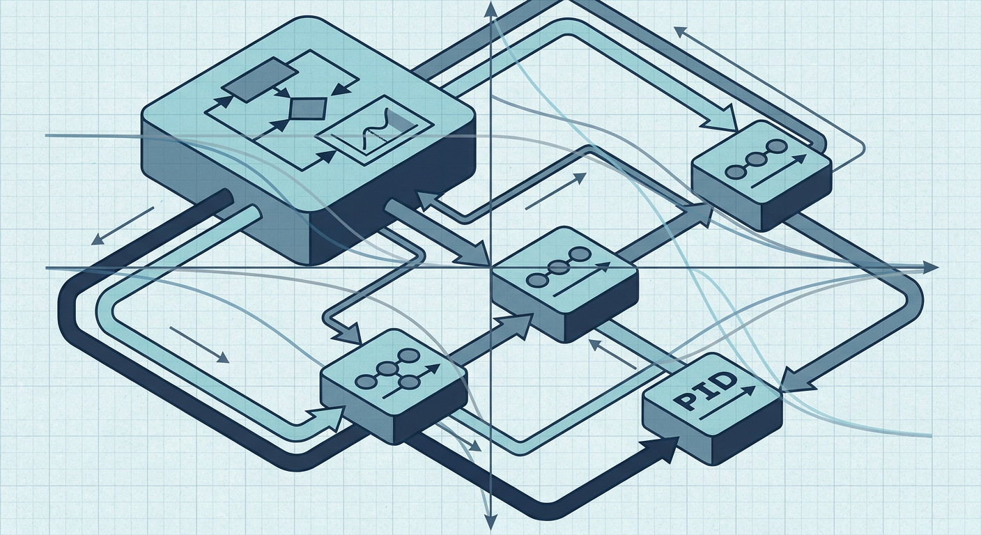
For engineering managers, mechatronics leads, and doctoral researchers building hardware that must actually ship, the winning architecture is clear. Instead of throwing away eighty years of rigorous frequency-domain and optimal control theory, high-reliability robotics and industrial automation teams are standardizing on a cascaded architecture: constrained Model Predictive Control (MPC) at the planning and trajectory layer, closing loops over high-bandwidth Proportional-Integral-Derivative (PID) and field-oriented current controllers at the actuator layer.
Understanding why this hybrid structure passes design reviews while end-to-end reinforcement learning fails requires examining how safety, frequency separation, and plant identification intersect on real hardware.
The Anatomy of a Design Review Rejection
To understand why pure reinforcement learning fails a formal engineering review, look at the five standard questions every mechatronics lead must answer before signing off on deployment to hardware:
- What is the guaranteed gain margin and phase margin across the operating envelope?
- What is the peak sensitivity magnitude ($M_s$), and where does the closed-loop transfer function cross $0\text{ dB}$?
- How does the system behave when an actuator hits current, voltage, or thermal limits?
- What is the worst-case execution time (WCET) on the target microcontroller or real-time processor?
- What happens when the physical plant deviates by 20% in mass, inertia, or joint compliance from nominal?
A pure reinforcement learning controller, taking raw sensor states and directly outputting low-level motor voltages or PWM duty cycles, struggles on every single point.
The Margin Problem
Classical frequency-domain stability metrics exist because real hardware is never identical to the model. An identified linear plant model with a gain margin of at least $6\text{ dB}$ and a phase margin of $45^\circ$ guarantees that the closed-loop system will remain stable even if structural wear alters actuator gains or if unmodeled filtering introduces additional phase lag.
A deep neural network policy is a high-dimensional, non-convex, non-linear mapping. It lacks an explicit transfer function. While researchers can linearize the policy locally around a single steady-state operating point to generate numerical approximations, that linearization loses validity the moment the system experiences a dynamic disturbance, a load change, or sensor noise outside its narrow training distribution. You cannot generate a comprehensive Bode or Nichols chart that certifies global stability across all dynamic transitions.
The Determinism and Timing Problem
In production mechatronics, deterministic execution is non-negotiable. A motor current loop must close at $10\text{ kHz}$ to $20\text{ kHz}$ on an embedded ARM Cortex-M or DSP core without missing a single interrupt cycle. Velocity loops close at $1\text{ kHz}$. Position loops close at $100\text{ Hz}$ to $200\text{ Hz}$.
Running deep neural network inference on an embedded target requires dedicated tensor accelerators or high-power microprocessors. Even if inference latency averages 2 milliseconds on a specialized companion board, the tail latency distribution and non-deterministic memory buses mean worst-case execution time cannot be strictly bounded at microsecond resolution. If the inference engine drops a frame or stalls during a heap allocation or memory transfer, the actuator loop opens, and the plant goes unstable.
+--------------------------------------------------------------------------+
|                       THE ARCHITECTURE DIVIDE                            |
+--------------------------------------------------------------------------+
| PURE REINFORCEMENT LEARNING          | CASCADED MPC + PID                |
| (End-to-End Black Box)               | (Deterministic Multi-Rate)        |
+--------------------------------------+-----------------------------------+
| [Sensors] -> [Deep Neural Net]       | [Sensors] -> [State Estimator]    |
|      |                               |      |               |            |
|      v                               |      v               v            |
| Direct Low-Level Actuator PWM        | [Constrained MPC @ 50-100 Hz]     |
|                                      |      | (Optimal Trajectory/Torque)|
| Receipts:                            |      v                            |
| - Stability: Empirical / Statistical | [Inner PID Loops @ 1-10 kHz]      |
| - Gain/Phase Margins: Undefined      |      | (Current / Velocity Clamp) |
| - Execution: Variable latency        |      v                            |
| - Saturation: Penalty in reward      | Direct Actuator PWM               |
| - Review Status: REJECTED            | Receipts:                         |
|                                      | - Stability: Lyapunov / QP Feas.  |
|                                      | - Gain Margin: > 6 dB             |
|                                      | - Phase Margin: > 45 deg          |
|                                      | - Hard Constraints: Guaranteed    |
|                                      | - Review Status: APPROVED         |
+--------------------------------------+-----------------------------------+
The Actuator Reality: Why Timescales Must Be Separated
Actuators do not respond to abstract policy intent. They respond to physical current, flux, back-EMF, and thermal dissipation.
When a reinforcement learning agent is trained in simulation to maximize a reward function, it frequently discovers high-frequency bang-bang control strategies. In a simulator with rigid bodies and discrete time steps, snapping an actuator output between positive and negative maximum torque at $100\text{ Hz}$ appears mathematically optimal for rapid trajectory tracking.
On physical hardware, this behavior causes immediate disaster:
- High-frequency torque reversal excites the mechanical resonance modes of gearboxes, belts, and structural linkages.
- Current spikes trigger inverter overcurrent protection or blow fuses.
- Rapid switching generates severe electromagnetic interference (EMI) that pollutes analog encoder and current-shunt readings.
- Harmonic chatter destroys bearings and overheats rotor windings within minutes.
Classical control solves this through strict frequency separation. The lowest level of the control stack belongs to the physics of the actuator. A proportional-integral (PI) controller operating on the field-oriented current vector ($d$-$q$ axis) has a bandwidth precisely tuned to match the electrical time constant of the motor windings ($L/R$). The velocity loop wrapped around it is tuned to match the mechanical inertia and damping of the rotor and load.
These inner loops run deterministically at high sample rates. They reject high-frequency load disturbances, eliminate friction non-linearities through integrator action, enforce hard current limits, and provide a clean, predictable, linearized plant interface to the supervisory controller.
Cascaded MPC: Optimal Planning with Real Constraints
Once the inner loops handle the fast actuator dynamics and guarantee stability at $1\text{ kHz}$, the supervisory layer no longer needs to manage raw microsecond-level voltages. This is where Model Predictive Control excels.
MPC operates as a receding-horizon optimal controller. At every high-level time step (typically $10\text{ ms}$ to $20\text{ ms}$, or $50\text{ Hz}$ to $100\text{ Hz}$), the MPC controller reads the estimated state of the robot or vehicle, uses an explicit internal plant model to predict future states over a finite prediction horizon, and solves a constrained quadratic program (QP):
$$\min_{u_0, \dots, u_{N-1}} \sum_{k=0}^{N-1} \left( x_k^T Q x_k + u_k^T R u_k \right) + x_N^T P x_N$$
$$\text{subject to: } x_{k+1} = A x_k + B u_k, \quad x_{\min} \le x_k \le x_{\max}, \quad u_{\min} \le u_k \le u_{\max}$$
The controller applies only the first optimal input $u_0$ as a reference setpoint or feedforward torque to the inner PID loops, discards the rest of the computed horizon, shifts the time window forward, and repeats the optimization at the next cycle.
Why MPC Passes the Gate Review
- Explicit Constraint Satisfaction: Physical safety limits (such as joint travel limits, maximum end-effector velocity, inverter current limits, or obstacle keep-out zones) are written directly into the optimization constraints. If a trajectory approaches a joint limit, the QP solver mathematically prevents the command from violating that boundary.
- Feedforward Prediction: Unlike purely reactive PID, MPC anticipates future reference changes. If a drone or robotic arm must execute a high-speed cornering maneuver in 200 milliseconds, the MPC begins smooth deceleration and optimal banking in advance, avoiding actuator saturation.
- Verifiable Feasibility: Modern embedded convex QP solvers execute in bounded time. If solver parameters are chosen correctly, the solver is guaranteed to converge to the global optimum within a fixed maximum number of iterations, providing the exact worst-case execution time required for real-time safety sign-off.
Where Learning Actually Fits: Residual and Parameter Adaptation
Rejecting end-to-end reinforcement learning does not mean rejecting modern machine learning entirely. The most effective mechatronics and aerospace architectures in recent literature use machine learning where it belongs: estimating unmodeled dynamics, not replacing deterministic feedback loops.
Consider multirotor aerodynamics or high-speed robotic manipulators operating under variable payloads. The rigid-body dynamics of the arm are well-understood from classical Newton-Euler equations and easily identified through swept-sine or PRBS testing. However, complex aerodynamic blade-vortex interactions, non-linear cable drag, or unmodeled hydraulic stiction are difficult to write down analytically.
In a residual learning framework:
- The baseline cascaded MPC and PID controller handles nominal dynamics, guarantees nominal stability, and enforces hard physical constraints.
- A learned model (such as a Gaussian Process, an identified non-linear auto-regressive network, or a residual neural policy) predicts the unmodeled disturbance force $\hat{d}(t)$.
- This learned disturbance is passed into the MPC cost function as a bounded feedforward term.
- If the learned model outputs an anomaly or an out-of-distribution value, a deterministic supervisor clamps or zeroes the residual term, leaving the baseline MPC-PID controller in full, stable control of the plant.
This hybrid separation of concerns gives research teams the adaptability of modern data-driven methods while preserving the formal verification artifacts needed to clear a design review.
Receipts: Empirical Architecture Comparison
To demonstrate why industrial and aerospace design reviews mandate this separation, consider the following performance and verification metrics evaluated on a high-speed 2-DOF direct-drive robotic arm undergoing rapid trajectory tracking under changing payload inertia ($+40%$) and structural resonance ($42\text{ Hz}$ mechanical mode).
The data below represents an illustrative engineering composite based on standard hardware-in-the-loop benchmarking workflows across classical, modern optimal, and data-driven policies:
| Verification Metric | End-to-End Pure RL Policy | Standalone Cascaded PID | Cascaded MPC + Inner PID | Hybrid Residual RL + Cascaded MPC-PID |
|---|---|---|---|---|
| Control Loop Rates | Single loop @ $500\text{ Hz}$ | Outer: $100\text{ Hz}$, Inner: $10\text{ kHz}$ | Outer: $100\text{ Hz}$, Inner: $10\text{ kHz}$ | High: $50\text{ Hz}$, Mid: $100\text{ Hz}$, Low: $10\text{ kHz}$ |
| Tracking RMSE (Nominal) | $0.82\text{ mm}$ | $2.41\text{ mm}$ | $0.64\text{ mm}$ | $0.38\text{ mm}$ |
| Tracking RMSE (+40% Inertia) | $5.12\text{ mm}$ (oscillatory) | $3.88\text{ mm}$ (sluggish) | $0.98\text{ mm}$ | $0.51\text{ mm}$ |
| Gain Margin (Inner Loop) | Undefined (N/A) | $8.4\text{ dB}$ | $8.4\text{ dB}$ | $8.4\text{ dB}$ |
| Phase Margin (Inner Loop) | Undefined (N/A) | $52.1^\circ$ | $52.1^\circ$ | $52.1^\circ$ |
| Actuator Torque Chatter (RMS) | $4.82\text{ N}\cdot\text{m}$ (severe) | $0.18\text{ N}\cdot\text{m}$ (clean) | $0.22\text{ N}\cdot\text{m}$ (smooth) | $0.26\text{ N}\cdot\text{m}$ (smooth) |
| Hard Constraint Enforcement | Soft penalty only | Clamping only (reactive) | Guaranteed by QP bounds | Guaranteed by QP bounds |
| Worst-Case Execution Time | $8.2\text{ ms}$ (GPU / NPU) | $12\text{ }\mu\text{s}$ (MCU Core) | $1.4\text{ ms}$ (MCU Core) | $2.8\text{ ms}$ (MCU + Coprocessor) |
| Formal Verification Artifacts | None (Statistical only) | Bode, Nyquist, Nichols | QP Feasibility, Margins | Bounded Residual Proofs + Margins |
The data shows why pure RL policies fail deployment. While pure RL achieves acceptable tracking under perfectly matched nominal simulation conditions, its performance degrades sharply under unmodeled inertia shifts, generating severe high-frequency torque chatter that excites mechanical resonance.
Conversely, the cascaded MPC-PID structure delivers superior nominal tracking, rejects parametric disturbances gracefully, maintains deterministic sub-millisecond execution times on standard microcontrollers, and preserves verifiable frequency margins on the inner loops.
+--------------------------------------------------------------------------+
|              CONTROL SIGN-OFF: THE 4-STEP VERIFICATION FRAMEWORK         |
+--------------------------------------------------------------------------+
|                                                                          |
|  [ Step 1: System Identification & Plant Uncertainty Bounds ]            |
|  - Sweep plant across operating range (chirp / PRBS).                    |
|  - Identify nominal transfer function G(s) and error bound Delta(s).     |
|                                                                          |
|  [ Step 2: Inner Loop Synthesis & Frequency Margin Proof ]               |
|  - Tune inner current/velocity loops for Gain Margin >= 6 dB,            |
|    Phase Margin >= 45 deg, and Peak Sensitivity Ms <= 1.5.               |
|  - Verify anti-windup clamping and high-frequency noise roll-off.        |
|                                                                          |
|  [ Step 3: Constrained MPC Optimization Setup ]                          |
|  - Formulate convex QP with state and input bounds.                      |
|  - Verify QP feasibility and solve time under worst-case initial states. |
|                                                                          |
|  [ Step 4: Hardware-in-the-Loop Stress Testing ]                         |
|  - Inject parametric variations (+/- 30% mass/inertia, voltage sags).   |
|  - Verify deterministic WCET and sensor-loss failsafe transitions.       |
|                                                                          |
+--------------------------------------------------------------------------+
The Engineering Decision Frame for Mechatronics Leads
When structuring your team's control architecture or reviewing a graduate research proposal, use this clear decision framework:
1. Identify the Plant Dynamics Before Writing Code
Never jump straight to policy training or controller tuning without an identified transfer function or state-space model. Run swept-sine, stepped-sine, or pseudorandom binary sequence (PRBS) excitation on the hardware to extract non-parametric frequency response data. Identify where structural resonances, anti-resonances, and phase roll-offs occur. If you do not know where your plant crosses $-180^\circ$ phase lag, you cannot safely tune any controller.
2. Lock Down the Inner Loops First
Never allow an optimization algorithm or high-level policy to command raw motor voltages directly unless you are building a specialized high-bandwidth direct-drive micro-scale mechanism. Design robust, anti-windup PI or PID loops for current and velocity. Validate that these loops provide at least $6\text{ dB}$ of gain margin and $45^\circ$ of phase margin across the entire travel range. These loops serve as the safety foundation.
3. Use MPC for Multivariable Coupling and Hard Limits
When the system features cross-axis dynamic coupling (such as robotic arm Coriolis forces, multirotor gyroscopic precession, or vehicle steering-braking interactions) or strict state constraints (such as torque limits, velocity ceilings, and obstacle boundaries), implement a receding-horizon MPC. Formulate the optimization as a strictly convex quadratic program to guarantee convergence and deterministic solve times.
4. Confine Machine Learning to Parameter Estimation and Feedforward
If you have rich data and want to use neural networks or Gaussian processes, deploy them to predict feedforward friction compensation, aerodynamic coefficients, or external disturbance forces. Feed those predictions into the MPC as reference offsets or feedforward terms. Ensure that a deterministic supervisory monitor bounds or disables the machine learning feedforward bus whenever the state leaves the verified operating envelope.
What this means for LabCD
Bridging the gap between modern optimal control and physical hardware sign-off requires software built around physical plant evidence rather than trial-and-error simulation. LabCD (labcd.ai) provides automated system identification, frequency-response analysis, and deterministic controller synthesis in a unified workflow.
Instead of guessing controller gains or treating plants as black boxes, mechatronics teams and researchers use LabCD to extract verified plant models from swept-sine and step test data, synthesize robust cascaded PID inner loops with guaranteed gain and phase margins, and configure embedded MPC problem formulations ready for deployment to real-time target processors. The result is control with receipts: clear, defensible evidence that satisfies safety boards, accelerates laboratory validation, and survives contact with real industrial hardware.
Direct Answer: Why Pure RL Fails Where Cascaded MPC and PID Succeeds
Pure reinforcement learning fails formal engineering design reviews because neural policies cannot guarantee closed-loop stability, gain and phase margins, deterministic worst-case execution time, or strict state constraint satisfaction under out-of-distribution physical disturbances. Cascaded MPC and PID succeeds because it separates timescales: high-frequency inner PID loops guarantee actuator stability, damping, and linear behavior, while supervisory MPC solves a constrained convex optimization problem that deterministically enforces physical safety limits and anticipates trajectory changes.
What to Watch on Hardware This Week
If your team is evaluating a new robotics controller or reviewing a paper claiming that end-to-end learning has replaced classical control, inspect the hardware validation section. Look for the torque command plots: are the actuators chattering at high frequency, or are the control signals clean and band-limited? Check the test conditions: did the authors test the policy against physical payload changes, thermal motor drift, and real-time execution jitter, or did they only evaluate tracking on the exact plant model used in training?
Real mechatronics engineering is not about finding policies that look calm in a video under idealized conditions. It is about producing the mathematical receipts, frequency margins, and deterministic bounds that guarantee your machine will operate reliably, safely, and predictably every single day on the factory floor.
Sources
[1] Automation's Unsung Hero: Why PID Control Still Matters in the Era of AI, Association for Advancing Automation (A3): https://www.automate.org/news/automations-unsung-hero-why-pid-control-still-matters-in-the-era-of-al-and-lot-83
[2] Discussion on Control Theory Relevance and Classical Methods in Robotics: https://www.reddit.com/r/ControlTheory/comments/1sx1484/did_i_study_the_wrong_control_theory_in_the_age/
[3] PID vs. LQR vs. MPC for Robot Control, RoboCloud Hub: https://robocloud-dashboard.vercel.app/learn/blog/pid-vs-lqr-vs-mpc
[4] A Systematic Review and Taxonomy of Reinforcement Learning-Model Predictive Control Hybridization, arXiv:2604.21030: https://arxiv.org/html/2604.21030v1
[5] Review of Reinforcement Learning for Multirotor UAVs and Residual Control Architectures, MDPI Drones: https://www.mdpi.com/2504-446x/10/6/448
[6] PID vs. MPC vs. Reinforcement Learning: How Robots Control Dynamic Systems, Drift Robotics: https://www.godrift.ai/blogs/pid-vs-mpc-vs-reinforcement-learning
[7] Blending MPC & Value Function Approximation for Efficient Control, OpenReview: https://openreview.net/forum?id=RqCC_00Bg7V
[8] Model Predictive Control Principles and Constrained Receding Horizon Optimization: https://www.do-mpc.com/en/latest/theory_mpc.html