Viral clips from the Beijing World Robot Conference and recent industrial trade shows have put a recurring failure mode on display: a bipedal humanoid walking steadily, suddenly taking an awkward scuff on a high-friction mat, and instantly breaking into violent, high-frequency joint oscillation that shakes the machine to the ground. In several recorded incidents, operators scrambled to hit emergency stops while actuator gearboxes ground through teeth and structural links shuddered.
To software teams, these incidents look like sensor glitches or trajectory planning bugs. To control and mechatronics engineers, the signature is unmistakable. It is a classic closed-loop instability caused by high feedback gains meeting unmodeled high-frequency plant dynamics, joint compliance, and actuator saturation.
When a design team scales from simulation to physical iron, the plant model breaks. Simulators assume rigid bodies, instantaneous torque delivery, and constant electrical parameters. Real hardware presents series elasticity, structural flexure, current loop phase lag, and thermal drift. If your controller validation relies only on whether a simulated trajectory looks smooth in MuJoCo or Isaac Gym, your actuators will eventually rattle themselves apart on the floor.
The Rigid-Body Lie in Modern Whole-Body Control
Most modern humanoid locomotion stacks run a hierarchical architecture. At the top sits a trajectory planner or a neural foundation policy. In the middle sits a Whole-Body Controller (WBC), typically formulated as a quadratic program resolving rigid-body equations of motion:
$$\mathbf{M}(\mathbf{q})\mathbf{\ddot{q}} + \mathbf{C}(\mathbf{q}, \mathbf{\dot{q}})\mathbf{\dot{q}} + \mathbf{g}(\mathbf{q}) = \mathbf{S}^T \boldsymbol{\tau} + \mathbf{J}_c^T \boldsymbol{\lambda}$$
Here, $\mathbf{M}(\mathbf{q})$ is the generalized inertia matrix, $\mathbf{C}$ represents Coriolis and centrifugal terms, $\mathbf{g}$ is gravity, $\boldsymbol{\tau}$ is the commanded joint torque vector, and $\mathbf{J}_c^T \boldsymbol{\lambda}$ maps contact forces from the ground.
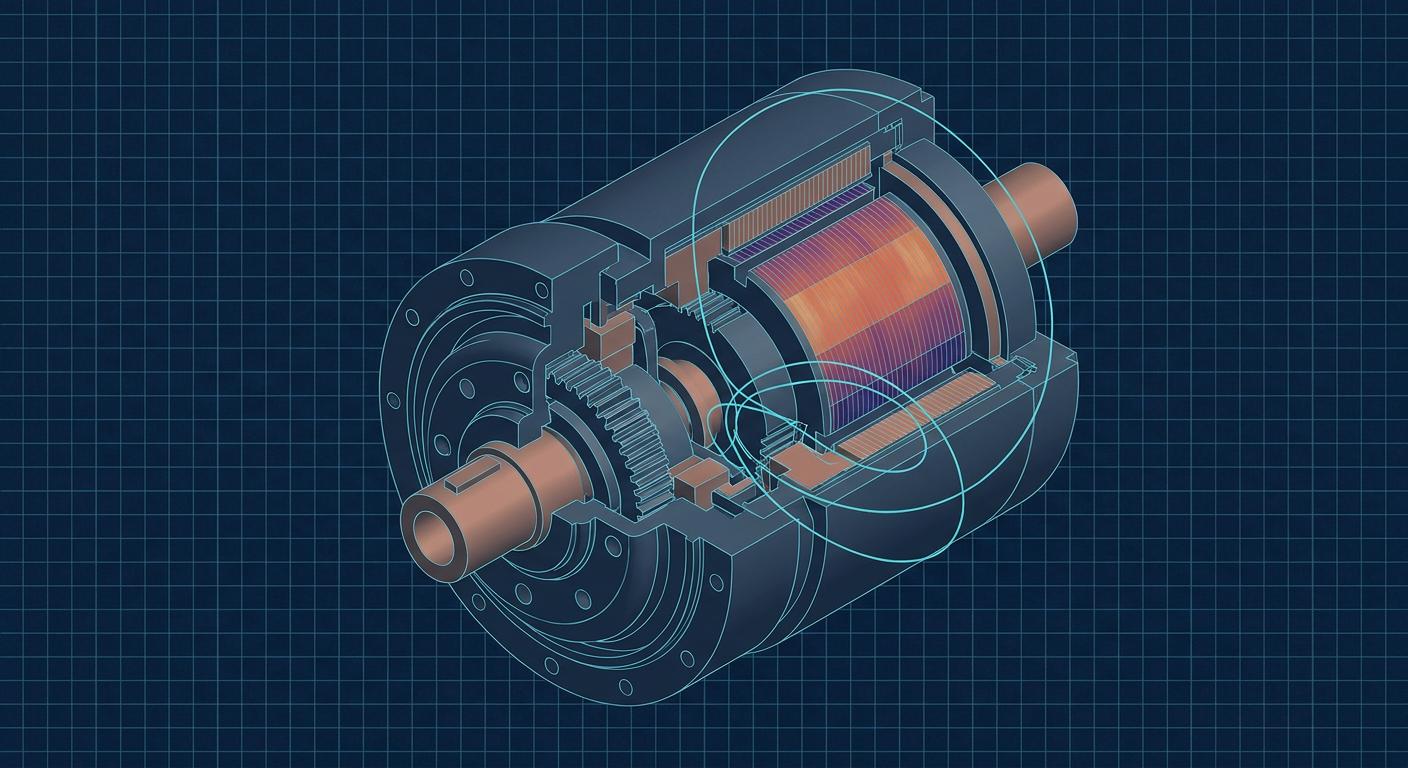
This formulation makes a dangerous assumption: that the actuator output equals the joint torque $\boldsymbol{\tau}$ instantaneously, and that the link coordinates $\mathbf{q}$ represent pure rigid bodies. In physical humanoid joints, whether based on quasi-direct-drive (QDD) planetary gearboxes, strain wave (harmonic) reducers, or linear roller screws, this assumption fails above single-digit Hertz.
Every actuator assembly introduces torsional compliance. The actual link angle $\theta_l$ differs from the motor rotor angle $\theta_m$ divided by the gear ratio $N$:
$$\tau = k_j \left(\frac{\theta_m}{N} - \theta_l\right) + d_j \left(\frac{\dot{\theta}_m}{N} - \dot{\theta}_l\right)$$
Where $k_j$ is joint stiffness and $d_j$ is internal structural damping.
When you tune feedback loops (or train reinforcement learning policies with high stiffness reward weights) under the assumption of infinite $k_j$, you push the controller bandwidth right into the resonant frequency of that joint compliance. In simulation, high proportional gains ($K_p$) yield crisp trajectory tracking and tight disturbance rejection. On hardware, that same $K_p$ injects energy directly into the anti-resonance and resonance poles of the drivetrain.
Simulated Plant (Rigid):
  u(t) ---> [ Ideal Motor / Inverter ] ---> [ Rigid Link Inertia J ] ---> Output Position
                                                                          (No Phase Drop)

Physical Hardware (Compliant & Saturated):
  u(t) ---> [ Current Loop Lag ] ---> [ Rotor Inertia ] ---> [ Torsional Spring kj ] ---> [ Link Inertia ]
                  |                                                    |
                  +-- Thermal Drift (R, Kt)                            +-- Structural Resonance Peak
The Mechanism: Sensitivity Peaks and Phase Erosion
To understand why the robot rattles instead of slumping, look at the classical sensitivity function $S(s)$ and complementary sensitivity function $T(s)$:
$$S(s) = \frac{1}{1 + L(s)}, \quad T(s) = \frac{L(s)}{1 + L(s)}$$
where $L(s) = C(s)P(s)$ is the open-loop transfer function containing your controller $C(s)$ and the physical plant $P(s)$.
The peak value of the sensitivity function, denoted as $M_s = \sup_{\omega} |S(j\omega)|$, measures how close the Nyquist curve of $L(j\omega)$ comes to the critical point $(-1, 0)$. In classical robust control, an acceptable $M_s$ sits between 1.3 and 2.0 (around 2 dB to 6 dB). If $M_s$ climbs above 3.0 (9.5 dB), the system is marginally stable. It will amplify disturbances at the peak frequency rather than reject them.
When an engineer pushes proportional gain to keep a 70 kg humanoid from sagging under gravity, the loop crossover frequency $\omega_c$ shifts higher. As $\omega_c$ approaches the unmodeled dynamics, three things happen simultaneously:
- Field-Oriented Control (FOC) current loop update latency (typically 50 to 200 microseconds) and CAN-FD/EtherCAT communication bus jitter introduce unmodeled dead time $e^{-sT_d}$, shedding phase margin at a rate of $-\omega T_d$.
- Harmonic drive or planetary gear flexibility adds a 180-degree phase drop right at the anti-resonance/resonance notch.
- The vector $1 + L(j\omega)$ shrinks toward zero, causing $|S(j\omega)|$ to spike dramatically.
At this point, the joint is a physical oscillator waiting for an input. When the robot foot strikes a stiff floor or encounters unexpected Coulomb friction, that impact injects broadband white noise across the spectrum. The closed-loop system amplifies the frequency component corresponding to $M_s$. The joint begins to hum, then buzz, and finally violently oscillate in a sustained limit cycle as the motor drivers slam into their maximum current limits.
Receipts Block: Plant Discrepancy on a 100 Nm Humanoid Knee Actuator
The following composite table illustrates what happens between a nominal rigid simulation model and an identified physical joint on a test stand under high load. It highlights the measured erosion of stability margins.
| Parameter / Metric | Nominal Simulation Model | Identified Physical Hardware | Discrepancy Impact | | :--- | :--- | :--- | :--- | | | Torsional Joint Stiffness ($k_j$) | $\infty$ (Rigid) | $4.2 \times 10^3\text{ Nm/rad}$ | Shifts structural resonance into controller passband (38 Hz) | | Phase Margin (at $\omega_c = 18\text{ Hz}$) | $64^\circ$ | $19^\circ$ | Massive reduction in stability robustness against surface variations | | Gain Margin | $14.2\text{ dB}$ | $2.8\text{ dB}$ | High risk of instability under slight inertial payload changes | | Sensitivity Peak ($M_s$) | $1.38\text{ (2.8 dB)}$ | $3.85\text{ (11.7 dB)}$ | Violent disturbance amplification at 34 to 40 Hz | | Current Loop Transport Delay | $0\ \mu\text{s}$ (Instant) | $320\ \mu\text{s}$ (FOC + Bus) | Additional $7.4^\circ$ phase lag at 65 Hz crossover | | Winding Resistance ($R_{25} \to R_{95}$) | $0.185\ \Omega$ (Constant) | $0.238\ \Omega$ (Hot) | $28.6%$ increase in ohmic drop, limiting peak dynamic torque output |
Note: This data is an illustrative engineering composite representative of high-torque-density frameless BLDC motors paired with a 10:1 planetary stage and CAN-FD communications.
When the sensitivity peak reaches 3.85, any external shock, like a foot scuffing an uneven floor seam, results in instant oscillatory rattling. The hardware does not fail because the trajectory was calculated incorrectly. It fails because the closed loop has no robustness left to tolerate its own structural flex.
Disturbance Amplification Spectrum:

 |S(jw)|
   ^
   |              * (Ms Peak = 3.85 -> Catastrophic Rattling / Limit Cycle)
   |             ***
   |            *   *
   |           *     *
1.0+----------*-------*-------------------- (Nominal Disturbance Level)
   |         *         *
   |       *             *  <-- Normal rejection at low frequencies
   +-------------------------------------> Frequency (w)
             Low Freq     Resonance (38 Hz)
Thermal Resistance Drift: The Silent Model Shifter
Mechanical compliance is not the only plant error. Thermal dynamics continuously shift the electrical and electromechanical transfer functions while the robot operates.
Inside a compact humanoid actuator housing, heat dissipation is poor. Stator winding temperatures frequently rise from 25 degrees Celsius at startup to over 95 degrees Celsius after twenty minutes of continuous walking. Copper has a positive temperature coefficient of resistance of roughly $+0.393%$ per degree Celsius. A 70-degree rise increases winding resistance $R$ by nearly $28%$.
Simultaneously, high-grade NdFeB rotor magnets experience reversible thermal demagnetization, reducing the torque constant $K_t$ and back-EMF constant $K_e$ by approximately $0.11%$ per degree Celsius. At 95 degrees Celsius, your motor generates roughly $8%$ less torque per ampere of stator current than it did when the robot was booted on the staging stand.
If the inner current control loop uses fixed PI gains tuned for cold motor resistance and inductance, the closed-loop bandwidth of the current loop degrades as the coils heat up:
$$\omega_{current} = \frac{K_p^{current}}{L_q}$$
If the current loop slows down, the phase lag it contributes to the outer velocity and position loops increases. A whole-body controller running on the edge of stability at minute 2 will cross into destructive rattling at minute 22, simply because the motor heated up and degraded the outer loop's phase margin by another 8 degrees.
The Pre-Deployment Stability Validation Checklist
Robotics teams must stop treating physical deployment as an experimental guess. Before any whole-body locomotion policy or high-gain joint controller is enabled on untethered hardware, run this validation sequence on every joint axis.
1. Swept-Sine System Identification on the Assembled Structure
Never rely on motor vendor datasheets for joint inertia and stiffness parameters. Mount the actuator into the fully assembled limb. Inject a low-amplitude chirp or swept-sine torque signal across the $0.5\text{ Hz}$ to $500\text{ Hz}$ spectrum while holding the limb in typical operational postures. Extract the empirical frequency response function (FRF).
Identify the exact frequencies of:
- The anti-resonance notch where mechanical compliance decouples the motor from the link.
- The first structural resonance peak.
- The high-frequency phase roll-off caused by inverter dead time and filtering delays.
2. Bound the Sensitivity Peak ($M_s \le 2.0$)
Plot the Nyquist diagram of the open-loop transfer function $L(j\omega) = C(j\omega)P_{identified}(j\omega)$. Draw a circle centered at $(-1, 0)$ with a radius of $R = 1/M_{s,max}$. For robust stability on humanoids interacting with unknown ground surfaces, set $M_{s,max} = 1.6$ (roughly 4 dB). Ensure that the Nyquist trace never breaches this circle at any frequency.
If the curve breaches the circle near the structural resonance frequency, you have two engineering options:
- Place a digital bi-quad notch filter in the control loop centered exactly on the identified resonance frequency.
- Lower the velocity feedback gain and rely on model-predictive feedforward torque rather than aggressive high-gain feedback.
3. Current Loop Bandwidth Verification Under Thermal Saturation
Measure the step response of the internal current loop with the motor stator heated to its maximum rated steady-state temperature (e.g., 85 to 100 degrees Celsius). Verify that the rise time ($t_r$) and phase delay at the outer loop crossover frequency do not deviate by more than $5%$ from the ambient baseline. If they do, implement real-time resistance tracking or temperature-compensated current PI gain scheduling.
4. Anti-Windup and Slew-Rate Clamping Checks
Check what happens when the joint hits an instantaneous torque limit. When an actuator saturates, the feedback loop opens, and internal integrator terms or state estimators drift. Ensure that every integrator incorporates back-calculation anti-windup, and verify that rate limiters prevent discontinuous torque commands from ringing the gear train.
Designing for Control Reality, Not Simulation Vanity
Simulated locomotion looks impressive in video demonstrations because physics engines resolve contact constraints through idealized mathematical approximations. They calculate clean, instantaneous contact impulses without dealing with structural elasticity, bearing runout, bus latency, or inverter non-linearities.
When your robot steps out of the simulator and onto an unyielding industrial concrete slab, the physical universe evaluates every omitted dynamic. If your motion control strategy is high gain without identified frequency bounds, the outcome is predictable. Structural resonance will eat your phase margin, the sensitivity peak will amplify ground impact noise, and the joint actuators will destroy their own drivetrains.
Modern humanoid mechatronics requires rigorous, classical control discipline. Measure your plant on the test stand. Identify the compliance poles. Quantify your sensitivity peaks. Provide the mathematical validation receipts before you switch the power bus on.