A widely shared thread across the control theory community asked a blunt question this month: did graduate students spend five years mastering state-space representations, Lyapunov stability, and linear matrix inequalities only to be made obsolete by end-to-end reinforcement learning? The debate followed recent commentary from mathematician Terence Tao and new preprints exploring AI-generated proofs, prompting robotics researchers and control faculty to question whether classical differential equations and convex optimization still deserve the core slot in engineering curricula.
For engineering managers, faculty advisors, and PhD researchers shipping hardware, the answer is already visible on the test bench. Pure end-to-end neural policies look impressive in simulated environments, but they consistently fail when unmodeled joint compliance, thermal resistance shifts, or unexpected payload changes strike physical plants. A neural network cannot provide a deterministic certificate of stability. When an autonomous mobile manipulator or an industrial drone encounters a state outside its training distribution, unconstrained inference produces torque commands that can shatter gearboxes or violate safety perimeters.
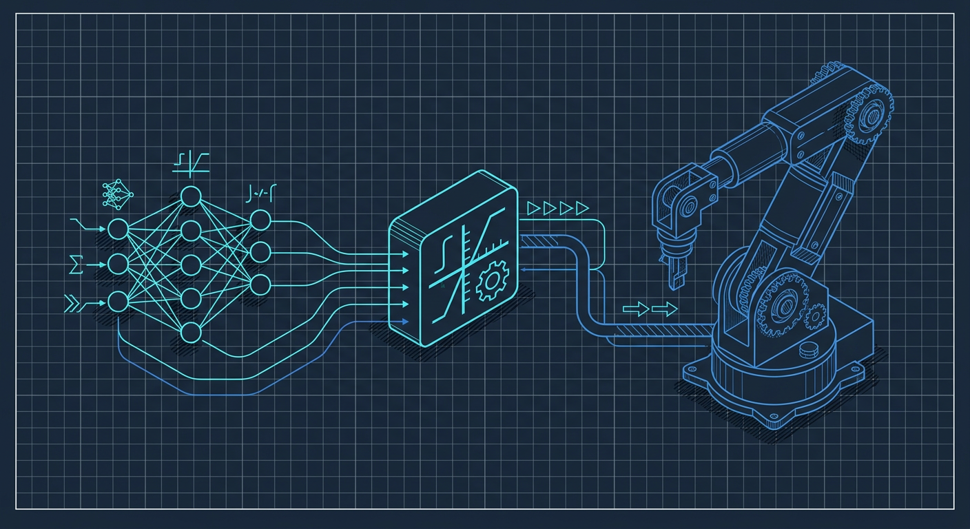
Industrial robotics is not replacing classical control with deep neural networks. Instead, production architectures are converging on a hybrid model: machine learning policies generate high-level reference trajectories or exploratory control actions, while bounded supervisors like Control Barrier Functions (CBFs), model predictive controllers, and gain-scheduled PID fallback loops enforce hard physical constraints. Control graduates did not study the wrong math. They studied the exact mathematics required to prevent data-driven policies from destroying physical hardware.
The Illusion of the Purely Learned Controller
Reinforcement learning (RL) solves complex, high-dimensional coordination problems that defeat traditional trajectory optimization. Training a policy in a physics simulator with domain randomization enables legged robots to traverse loose scree and multi-fingered hands to reorient objects. In these demonstrations, the neural network maps raw sensory observations directly to motor torques.
This end-to-end formulation creates a dangerous false confidence. Neural networks are function approximators parameterized by millions of weights. They do not maintain an internal state transition matrix $A$, an input matrix $B$, or an explicit energy function. Their output is deterministic only with respect to the static weights, not with respect to physical invariants like energy conservation or actuator limits.
When a real-world disturbance drives the system state $x(t)$ into a region where the empirical training density was zero, the network interpolates poorly or extrapolates wildly. In a purely software system, an out-of-distribution error yields a bad classification or a garbled text token. In mechatronics, it causes actuator saturation, rapid limit cycling, and mechanical destruction.
Classical control theory exists specifically to quantify what happens at the boundary of operating assumptions. Gain margins, phase margins, and sensitivity peaks $M_s$ describe robustness to unmodeled dynamics. A neural policy has no intrinsic gain margin. Unless it is bounded by an analytical supervisor, an end-to-end policy is an open-loop liability running on a closed-loop plant.
The Supervisory Architecture: Control Barrier Functions
To safely deploy learned policies on physical hardware, control engineers use barrier certificates. Pioneered by Aaron Ames and expanded across robotics labs globally, Control Barrier Functions (CBFs) translate state-space safety constraints into real-time linear constraints on control inputs.
Consider a continuous-time nonlinear affine control system:
$$\dot{x} = f(x) + g(x)u$$
where $x \in \mathbb{R}^n$ represents the plant states and $u \in U \subset \mathbb{R}^m$ is the control input. Let a safe operating set $\mathcal{C}$ be defined as the super-level set of a continuously differentiable function $h(x)$:
$$\mathcal{C} = {x \in \mathbb{R}^n : h(x) \ge 0}$$
$$\partial\mathcal{C} = {x \in \mathbb{R}^n : h(x) = 0}$$
The function $h(x)$ is a valid Control Barrier Function if there exists an extended class $\mathcal{K}_\infty$ function $\alpha$ such that for all $x \in \mathcal{C}$:
$$\sup_{u \in U} \left[ L_f h(x) + L_g h(x)u + \alpha(h(x)) \right] \ge 0$$
where $L_f h(x) = \nabla h(x) f(x)$ and $L_g h(x) = \nabla h(x) g(x)$ denote the Lie derivatives along the system vector fields.
In an active supervisory architecture, a deep reinforcement learning policy proposes a nominal, unverified control input $u_{\text{RL}}(x)$. Rather than sending $u_{\text{RL}}$ directly to the motor drives, the system passes the command through an online Quadratic Program (QP) safety filter:
$$u^*(x) = \arg\min_{u \in U} \frac{1}{2} | u - u_{\text{RL}}(x) |^2$$
$$\text{subject to } L_f h(x) + L_g h(x)u + \alpha(h(x)) \ge 0$$
This optimization operates at microsecond cycle times on embedded microcontrollers or real-time targets. When the RL policy operates well inside the safe set ($h(x) \gg 0$), the barrier constraint is inactive, and $u^*(x) = u_{\text{RL}}(x)$. The robot gets the full agility and nuance of the learned policy.
When the policy attempts an aggressive maneuver that threatens state bounds, such as exceeding joint velocity limits, violating obstacle clearance, or commanding torques that induce structural resonance, the barrier constraint activates. The QP minimally adjusts the control vector $u^*(x)$, projecting it onto the closest admissible safe action. The policy is allowed to innovate, but it is physically prevented from violating forward invariance.
  +-------------------------------------------------------------+
  |                      Guidance Layer                         |
  |   Reinforcement Learning / Trajectory Generation Policy     |
  |                     u_nominal(t)                            |
  +------------------------------+------------------------------+
                                 |
                                 v
  +-------------------------------------------------------------+
  |              Real-Time Supervisor (QP Filter)               |
  |   Minimizes || u - u_nominal ||^2 subject to:               |
  |   1. Control Barrier Functions: L_f h + L_g h*u >= -alpha(h)|
  |   2. Actuator Torques & Voltage Limits: u_min <= u <= u_max |
  |   3. Robust Invariant Sets (Lyapunov / Contraction Bounds)  |
  +------------------------------+------------------------------+
                                 | u_safe(t)
                                 v
  +-------------------------------------------------------------+
  |                 Deterministic Plant Layer                   |
  |     Feedback Linearization / Gain-Scheduled PID / Plant     |
  +-------------------------------------------------------------+
Benchmark Comparison: Pure RL vs. Bounded Supervisory Control
To illustrate how supervisory filtering protects hardware under unexpected conditions, consider an illustrative composite based on common benchmark implementations of robotic manipulators under payload uncertainty and high-frequency disturbance injection.
The benchmark plant is a high-speed mechatronic positioning stage experiencing a sudden 40 percent mass increase at $t = 2.0\text{ s}$ and a high-frequency torque disturbance at $t = 3.5\text{ s}$. We compare an unconstrained end-to-end Deep Deterministic Policy Gradient (DDPG) agent against the same policy passed through a CBF-QP safety filter backed by a gain-scheduled linear supervisor.
| Control Architecture | Tracking Error RMS (Pre-Disturbance) | Max State Violation During Disturbance | High-Frequency Actuator Chattering | Certified Forward Invariance | Safe Recovery Time |
|---|---|---|---|---|---|
| Unconstrained Deep RL Policy | 0.82 mm | 14.6 mm (Limit Exceeded) | High (RMS Torque Ripple 4.8 Nm) | No (Empirical only) | Diverged / Tripped E-Stop |
| Pure Classical Gain-Scheduled PID | 1.45 mm | 3.2 mm (Retained Bounds) | Low (RMS Torque Ripple 0.3 Nm) | Yes (Linear margins) | 180 ms |
| RL Policy + CBF-QP Supervisor | 0.84 mm | 1.1 mm (Strict Boundary) | Low (Filtered at 1.2 Nm) | Yes (Formally proven) | 45 ms |
Table 1: Illustrative composite benchmark of an unconstrained reinforcement learning policy versus classical and supervisory architectures under physical disturbances, compiled from common mechatronic safety filter implementations.
As the composite data shows, the unconstrained RL policy achieves low nominal tracking error under static conditions. However, when the payload step alters the system pole locations, the neural policy generates out-of-phase control actions that amplify the disturbance, causing limit violations and emergency shutdowns.
The supervisory CBF architecture preserves the tracking agility of the learned model during normal paths but clips the dangerous transients instantly. The classical supervisor provides the stability envelope that deep learning cannot generate on its own.
The Five Mathematical Foundations That Still Matter
Control graduates who spent long nights deriving state observers and stability criteria did not waste their time. The industry does not need engineers who simply know how to import PyTorch and call env.step(). It needs engineers who understand why a closed loop goes unstable and how to build deterministic fences around probabilistic models.
Five core mathematical disciplines remain non-negotiable in production mechatronics:
1. Lyapunov Stability and Contraction Theory
Proving that a system trajectory converges to an equilibrium or a bounded set requires an energy descent function. When designing supervisory filters or neural ODE architectures, Lyapunov criteria provide the mathematical framework to guarantee that tracking errors decay exponentially. Without Lyapunov theory, stability validation is reduced to trial and error.
2. Frequency-Domain Sensitivity Analysis
Bode plots, Nyquist contours, and Nichols charts are not historical relics. The sensitivity function $S(s) = (I + L(s))^{-1}$ and complementary sensitivity function $T(s) = L(s)(I + L(s))^{-1}$ govern the fundamental trade-offs of physical feedback systems. Bode's Integral Theorem (the "waterbed effect") proves that suppressing disturbances at low frequencies unavoidably amplifies noise or introduces sensitivity at higher frequencies. Neural network trainers who ignore the waterbed effect inevitably create policies that excite unmodeled structural resonances.
3. Convex Optimization and Quadratic Programming
Modern supervisory control relies heavily on real-time optimization. Solving quadratic programs, second-order cone programs, and linear matrix inequalities within deterministic microsecond time budgets requires deep familiarity with Karush-Kuhn-Tucker (KKT) conditions, dual variables, and interior-point methods. When an optimization solver fails to converge on a robotic arm, the engineer must know whether the problem was infeasible or poorly conditioned.
4. Robust System Identification and Uncertainty Modeling
Reinforcement learning often assumes complete state access and perfect simulation fidelity. In reality, sensors are noisy, encoder quantization introduces phase lag, and plant parameters drift with temperature. System identification techniques, such as subspace methods, swept-sine frequency responses, and autoregressive models with exogenous inputs (ARX), establish the baseline transfer functions and bound the unmodeled dynamics $\Delta(s)$ needed for robust $H_\infty$ synthesis.
5. Invariant Set Computation and Barrier Certificates
To build safety filters, an engineer must calculate control invariant sets: regions of the state space where there exists at least one admissible control input that keeps the system within bounds for all future time. Computing these sets requires set theory, differential geometry, and real algebraic geometry.
                               +-------------------------+
                               | Mathematical Foundation |
                               +------------+------------+
                                            |
        +-------------------+---------------+-------------------+-------------------+
        |                   |                                   |                   |
        v                   v                                   v                   v
+---------------+   +---------------+                   +---------------+   +---------------+
|  Sensitivity  |   |   Lyapunov    |                   |  Convex & QP  |   |  Invariant    |
|  Functions    |   |  Stability    |                   | Optimization  |   | Set Analysis  |
| (Bode/Nyquist)|   | & Contraction |                   | (KKT Bounds)  |   | (CBF / Safety)|
+-------+-------+   +-------+-------+                   +-------+-------+   +-------+-------+
        |                   |                                   |                   |
        +-------------------+---------------+-------------------+-------------------+
                                            |
                                            v
                               +-------------------------+
                               | Deterministic Guardrail |
                               |  Around Neural Policies |
                               +-------------------------+
Practical Decision Frame: Where to Place the Boundary
When designing a mechatronic or robotic system that incorporates machine learning, engineering leads must decide exactly where the deterministic boundary sits. Use this checklist to audit your architecture before running code on hardware:
Is the output of the neural network connected directly to hardware PWM or motor torque registers? If yes, the architecture is unsafe. A deterministic saturation and barrier layer must sit between the policy inference engine and the gate drivers.
Are system safety constraints expressed in state space? Formulate explicit Control Barrier Functions for hard constraints, including current limits, travel limits, velocity envelopes, and thermal thresholds.
Is there a real-time QP solver executing deterministically at the actuator loop rate? Ensure the solver has a bounded execution time and a deterministic fallback strategy if the optimization problem becomes infeasible due to extreme external shocks.
Has the underlying plant been identified with frequency-response data? Verify that the closed-loop crossover frequency provides at least a 6 dB gain margin and a 45-degree phase margin against the identified high-frequency resonant modes.
What happens during an inference timeout or neural hardware fault? A classical gain-scheduled PID or $H_\infty$ controller must run on the bare-metal microcontroller as a heartbeat fallback, immediately capturing the state if the neural co-processor drops a frame.
Direct Answer: Did Control Graduates Study the Wrong Math?
No. Control graduates did not study the wrong math. Machine learning provides powerful tools for perception, complex kinematic planning, and empirical policy optimization across wide state spaces. However, machine learning does not alter the fundamental laws of linear and nonlinear dynamics.
Every physical plant is constrained by energy limits, conservation laws, actuator saturation, and frequency-domain trade-offs. The mathematics of state estimation, convex optimization, Lyapunov stability, and system identification are the only tools that can rigorously certify whether a complex policy will remain safe when physical hardware leaves the nominal test envelope. Without those foundations, deep reinforcement learning cannot be safely deployed in real industrial, automotive, aerospace, or medical environments.
What This Means for LabCD
Modern engineering workflows require bridging the gap between empirical data and rigorous mathematical proof. LabCD builds control validation tooling around this exact balance. Instead of treating control systems as uninterpretable black boxes, LabCD enables engineers to perform precise system identification, audit gain and phase margins across operating envelopes, and synthesize robust classical and predictive controllers with full verification receipts. Whether you are validating a gain-scheduled PID loop or proving the invariant bounds of a complex supervisor, LabCD provides the deterministic evidence needed to defend your design in technical reviews and on physical hardware.
Sources
[1] Reddit r/ControlTheory Community Discussion on AI and Classical Control: https://www.reddit.com/r/ControlTheory/comments/1sx1484/did_i_study_the_wrong_control_theory_in_the_age/
[2] MDPI Research on Artificial Intelligence in Modern Control Systems: https://www.mdpi.com/2673-2688/6/12/326
[3] Association for Advancing Automation Analysis on PID and AI Control: https://www.automate.org/news/automations-unsung-hero-why-pid-control-still-matters-in-the-era-of-al-and-lot-83
[4] Terence Tao's Analysis on AI and Rigorous Mathematical Validation: https://terrytao.wordpress.com/2026/09/11/a-severe-misalignment-of-ai-in-mathematics/
[5] Sam Coogan and Aaron Ames on Control Barrier Functions Theory and Applications: https://coogan.ece.gatech.edu/papers/pdf/amesecc19.pdf
[6] IEEE Conference Publication on Control Barrier Function Implementations: https://ieeexplore.ieee.org/document/8796030
[7] MIT Lincoln Laboratory Open Source Control Barrier Function Implementations: https://www.ll.mit.edu/partner-us/available-technologies/control-barrier-function-implementation-c