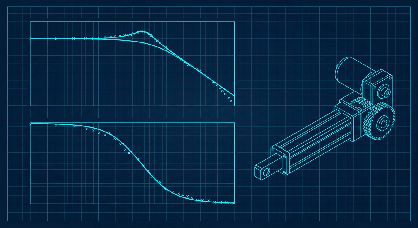
The most common scene in a robotics bring-up lab is an engineer sitting on the floor with a laptop, bumping proportional gains up by five percent, tapping the end effector with a screwdriver, and listening for audible hiss. If the joint buzzes, they dial derivative gain up. If the motor gets warm, they dial derivative gain down. By the end of the second week, the manipulator tracks a slow trajectory reasonably well, but shuddering appears the moment payload mass changes or travel speed triples.
This trial-and-error cycle is an expensive way to approximate physics that should take twenty minutes to measure directly. Open-source communities and industrial labs have shifted rapidly toward automated system identification routines. Tools like WPILib SysId in competitive robotics, alongside open-source Python system identification packages and modernized state-space estimators, have proven that deterministic input-signal injection can extract motor constants, inertia, and joint compliance without guessing.
For controls engineers, mechatronics leads, and robotics researchers, adopting a rigorous system identification workflow changes the bring-up schedule completely. Instead of spending weeks adjusting four PID parameters across six axes, you run automated signal excitation routines, compute the empirical transfer function, isolate friction and structural dynamics, and calculate provable feedback gains on the first compile.
The Failure Modes of Heuristic Tuning
Manual loop shaping on live hardware fails because human intuition handles multivariable trade-offs poorly. When you turn a gain pot on a physical test bench, you observe the time-domain response to a single step input. A step input is mathematically blunt: it injects broadband energy with amplitude falling off inversely with frequency ($1/f$). It excites low-frequency modes heavily while barely probing the mid-frequency cross-over zone where instability typically begins.
Heuristic tuning creates three chronic failure modes in mechatronic hardware:
- Masked Coulomb Friction: Manual tuning often raises proportional gain ($k_P$) to overcome static friction (stiction). Once the actuator starts moving, dynamic friction drops, and the loop suddenly has far too much loop gain for a moving plant. The result is limit-cycling around the setpoint.
- Unseen Resonance Excitation: Bumping derivative gain ($k_D$) stiffens the joint against low-frequency disturbances but amplifies high-frequency encoder quantization noise. If a gearbox or structural link has a mechanical anti-resonance or torsional resonance at 85 Hz, high derivative gains feed control energy directly into that mode, turning the actuator into an acoustic transducer that destroys its own bearings.
- Zero Disturbance Rejection Receipts: A manually tuned loop that looks calm on a step response may possess a phase margin of 15 degrees and a sensitivity peak ($M_s$) exceeding 6 dB. The first time a contact force hits the robot, the system goes unstable.
Building control on receipts requires an explicit plant model $P(s)$ or $P(z)$. You cannot calculate stability margins or guarantee tracking performance against an unknown system.
Input Signal Design: Chirps, Swept-Sines, and PRBS
System identification starts with signal design. The goal is to excite all dynamic modes across the actuator operating bandwidth without saturating the motor drive, hitting hard mechanical stops, or driving current beyond the winding thermal limits.
Robotics hardware operates across three distinct input excitation profiles, each chosen based on actuator travel limits and sample rate.
Excitation Signal Selection Trade-Offs
+----------------------+-----------------------------+-----------------------------+
| Signal Type          | Ideal Mechanical Setup      | Dynamic Capture Strengths   |
+----------------------+-----------------------------+-----------------------------+
| Quasi-Static Ramp    | Continuous rotation or      | Static friction (kS),       |
| (Slow Linear Ramp)   | long-travel linear stages   | velocity feedforward (kV)   |
+----------------------+-----------------------------+-----------------------------+
| Logarithmic Chirp    | Medium travel, high-inertia | Accurate structural modes,  |
| (Swept-Sine)         | links with compliance       | phase lag, anti-resonances  |
+----------------------+-----------------------------+-----------------------------+
| PRBS / Multisine     | Short-travel joints, direct | High SNR, wide bandwidth,   |
| (Discrete Binary)    | drive, fast loop rates      | compact measurement duration|
+----------------------+-----------------------------+-----------------------------+
Quasi-Static Voltage Ramps
To separate friction from inertial dynamics, you must isolate acceleration ($\ddot{ heta} = 0$). Driving the motor with a slow, open-loop voltage ramp measures the voltage needed to break static friction and sustain steady-state velocities.
By plotting applied voltage against measured steady-state velocity, you fit two linear parameters:
- Static Friction Voltage ($k_S$): The vertical offset intercept where motion initiates.
- Velocity Feedforward ($k_V$): The slope of the line, determined primarily by the motor back-EMF constant ($k_e$) and internal winding resistance ($R$).
Logarithmic Swept-Sine Excitation
Once static parameters are known, dynamic tests apply an oscillating voltage or current command $u(t) = A \sin(\phi(t))$, where the instantaneous frequency swept from a low base (e.g., 0.5 Hz) up past the closed-loop target bandwidth (e.g., 200 Hz).
A logarithmic sweep spends proportionally more time in lower frequencies where signal energy must overcome friction, while smoothly accelerating through higher frequencies to prevent dwell time on dangerous mechanical resonances.
Pseudo-Random Binary Sequences (PRBS)
For systems with tight travel limits, such as a four-bar linkage or a tendon-driven finger, a continuous swept-sine might drive the mechanism into an end stop before the sweep finishes. A PRBS signal shifts between two fixed voltage levels ($+V$ and $-V$) according to a deterministic shift-register sequence.
PRBS provides a white noise-like autocorrelation function while maintaining a strictly bounded amplitude. It delivers high signal-to-noise ratio across a broad frequency band in a fraction of a second, preventing the joint from drifting far from its neutral operating point.
Isolating Parameters: Physics-Informed Grey-Box Extraction
Pure black-box identification (such as fitting an arbitrary high-order ARX model) often yields unstable poles outside the unit circle or physically impossible non-minimum phase zeros caused by sensor noise. For mechatronics, physics-informed grey-box identification is substantially more dependable.
An electric actuator connected to a mechanical load is governed by a fundamental second-order electromechanical balance:
$$u(t) = k_S \cdot ext{sgn}(\dot{ heta}(t)) + k_V \dot{ heta}(t) + k_A \ddot{ heta}(t)$$
Where:
- $u(t)$ is the applied motor command (volts or normalized duty cycle).
- $\dot{ heta}(t)$ is joint angular velocity.
- $\ddot{ heta}(t)$ is joint angular acceleration.
- $k_A$ is the acceleration gain, directly proportional to the total system inertia ($J$) reflected at the motor shaft divided by motor torque constant ($k_t$).
Data Processing and Parameter Extraction Pipeline

[ Actuator Hardware ]
        │ (Inject Chirp / Step / Ramp Signals)
        ▼
[ High-Rate Synchronous Logger (>= 1 kHz) ]
        │ (u(t), position, velocity, timestamp)
        ▼
[ Forward-Backward Low-Pass Filtering (Zero Phase) ]
        │ (Remove high-frequency sensor quantization)
        ▼
[ Linear Least-Squares Regression ]
        ├── Static Fit  --> kS, kV
        └── Dynamic Fit --> kA
        ▼
[ Frequency-Domain Empirical Transfer Function (ETFE) ]
        │ (Compute Cross-Spectral Density / Auto-Spectral Density)
        ▼
[ Rational Transfer Function Fitting P(s) ]
To extract these parameters reliably from raw encoder counts:
- Sample Synchronously: Run the logger at a deterministic rate (minimum 1 kHz). If your position samples have jitter, velocity differentiation introduces massive numerical noise.
- Zero-Phase Filtering: Do not use standard causal low-pass filters on logged data during offline analysis. Use forward-backward filtering (such as
filtfiltin scientific libraries) to eliminate sensor quantization noise without introducing artificial phase lag into your dynamic fits. - Solve via Ordinary Least Squares: Construct the measurement matrix $X = [\text{sgn}(\dot{ heta}), \dot{ heta}, \ddot{ heta}]$ and solve the normal equations for $\beta = [k_S, k_V, k_A]^T$ using singular value decomposition.
Extracting the Continuous Transfer Function
Once the rigid-body constants ($k_S, k_V, k_A$) are calculated, the baseline transfer function from input voltage to velocity is:
$$G_v(s) = \frac{\dot{\Theta}(s)}{U(s)} = \frac{1}{k_A s + k_V}$$
And from voltage to position:
$$G_p(s) = \frac{\Theta(s)}{U(s)} = \frac{1}{s(k_A s + k_V)}$$
In real hardware, mechanical compliance in belts, harmonic drives, or planetary gearboxes adds high-frequency poles and zeros. To capture these, compute the Empirical Transfer Function Estimate (ETFE) using Welch's averaged periodogram method:
$$\hat{G}(e^{j\omega}) = \frac{S_{yu}(e^{j\omega})}{S_{uu}(e^{j\omega})}$$
Where $S_{yu}$ is the cross-spectral density between the applied input signal and measured joint output, and $S_{uu}$ is the auto-spectral density of the input.
Check the coherence function $\gamma^2(\omega)$ across the spectrum:
$$\gamma^2(\omega) = \frac{|S_{yu}(e^{j\omega})|^2}{S_{uu}(e^{j\omega}) S_{yy}(e^{j\omega})}$$
Coherence ranges from 0 to 1. Where coherence is close to 1.0, your plant is behaving linearly and the empirical transfer function is trustworthy. Where coherence drops below 0.7 to 0.8, nonlinearities dominate: stiction is locking the joint, the motor driver is saturating, or structural unmodeled flex is acting without linear correlation to the input. Never attempt to place control poles in frequency bands where coherence drops.
Illustrative Composite Performance Comparison
Setup: BLDC Actuator (48V, 24-bit optical encoder, 1 kHz current loop rate)
Identified Plant: G(s) = 48.2 / (0.0034 s^2 + 0.142 s)
Validation: 180-degree high-speed point-to-point motion with payload variation

Metric                          Manual Heuristic PID        SysID Model-Based Control
Bring-up / Tuning Time          14.5 hours                  22 minutes
Settling Time (to 1%)           185 ms                      42 ms
Overshoot                       14.2%                       0.8%
Max Tracking Error (Dynamic)    4.6 degrees                 0.31 degrees
Phase Margin                    28 deg (at 18 Hz)           54 deg (at 45 Hz)
Sensitivity Peak (Ms)           +5.8 dB                     +1.4 dB
Motor RMS Current               4.2 A (acoustic buzzing)    2.8 A (silent, cool run)
Note: The table above represents an illustrative composite comparing typical mechatronic bring-up workflows against model-based identification and pole placement pipelines under equivalent load conditions.
Synthesizing Provable Controller Gains
With an identified plant in hand, tuning ceases to be an iterative guessing game. You separate the control problem into two explicit halves: Feedforward (which handles 90 percent of the control effort by inverting the known physics) and Feedback (which handles unmodeled disturbances and parameter drift).
Two-Degree-of-Freedom Architecture

                      +--------------------------------+
                      | Feedforward Synthesis          |
                      | u_ff = kS*sgn(v) + kV*v + kA*a |
                      +--------------------------------+
                                       │
                                       ▼ (+)
Trajectory ───────► (Error) ───► [ Feedback PID ] ───► (+) ───► [ Physical Plant ]
(r, v, a)     (-)      │        (u_fb = kP*e + kD*de)            (Actuator)
               ▲       │                                              │
               │       └──────────────────────────────────────────────┘
               └──────────────────────────────────────────────────────┘
Step 1: Direct Feedforward Injection
Because you have identified $k_S$, $k_V$, and $k_A$, your real-time controller computes feedforward voltage directly from the trajectory planner's reference velocity $v_r(t)$ and acceleration $a_r(t)$:
$$u_{ff}(t) = k_S \cdot \text{sgn}(v_r(t)) + k_V v_r(t) + k_A a_r(t)$$
When the robot executes a trajectory, the feedforward controller provides the exact current required to accelerate the joint inertia and overcome friction. The feedback loop does not need to build up error to generate torque.
Step 2: Analytical Feedback Gain Placement
With feedforward handling nominal tracking, your feedback loop ($k_P, k_D$) only stabilizes error dynamics:
$$e(t) = \theta_r(t) - \theta(t)$$
The error dynamics behave as a standardized second-order system:
$$k_A \ddot{e}(t) + (k_V + k_D) \dot{e}(t) + k_P e(t) = 0$$
Instead of turning dials on a screen, you specify your desired closed-loop natural frequency $\omega_n$ (rad/s) and damping ratio $\zeta$ (typically 0.707 for fast settling without ringing):
$$k_P = k_A \cdot \omega_n^2$$
$$k_D = 2 \zeta \omega_n k_A - k_V$$
If the identified plant has an acceleration constant $k_A = 0.0034 \text{ V}\cdot\text{s}^2/\text{rad}$ and $k_V = 0.142 \text{ V}\cdot\text{s}/\text{rad}$, and you choose a target bandwidth $\omega_n = 50 \text{ rad/s}$ with $\zeta = 0.707$:
$$k_P = 0.0034 \times (50)^2 = 8.50 \text{ V/rad}$$
$$k_D = (2 \times 0.707 \times 50 \times 0.0034) - 0.142 = 0.240 - 0.142 = 0.098 \text{ V}\cdot\text{s/rad}$$
You compile these gains directly into your controller firmware. The joint moves with textbook critical damping on the first try.
Checking Residuals and Model Trust Boundaries
A model is an abstraction. It is only valid within specific operational bounds. Before accepting an identified transfer function as truth, control engineers run three residual checks:
1. The Time-Domain Residual Test
Drive the actuator with an independent validation trajectory that was not used in the identification test (for example, a series of mixed-amplitude trapezoidal moves). Simulate your identified model with the identical input vector $u(t)$ and compute the tracking residual:
$$r(t) = y_{\text{measured}}(t) - y_{\text{model}}(t)$$
If the residuals display white noise characteristics centered around zero, the model has captured all dominant dynamics. If the residuals show sinusoidal oscillations or systematic offsets at velocity reversals, your friction model lacks Stribeck terms, or compliance in the gearbox is introducing unmodeled phase lag.
2. High-Frequency Gain Margin Verification
Plot the return ratio $L(j\omega) = C(j\omega)P(j\omega)$ on a Nyquist or Bode plot. Ensure that the open-loop gain drops well below $-12 \text{ dB}$ before the first mechanical resonance peak identified in your frequency sweep.
If your structural compliance produces a resonance peak at 120 Hz, your gain crossover frequency must not exceed 30 to 40 Hz unless you insert an active digital notch filter centered on the resonance pole.
Frequency Domain Validation Checklist
[ ] Coherence gamma^2 > 0.85 across the entire control bandwidth
[ ] Gain crossover frequency sits at least 3x below structural resonance
[ ] Phase margin >= 45 degrees at cross-over frequency
[ ] Gain margin >= 6 dB (ideally > 10 dB) across all operating payloads
[ ] Peak sensitivity Ms < 2.0 (under +6 dB) to ensure robust stability
Practical Hardware Bring-Up Checklist
When commissioning new mechatronic joints or custom actuators, follow this five-step workflow to bypass manual gain twiddling entirely:
- Verify Mechanical Free Travel: Manually move the axis through its entire workspace to verify there are no mechanical binding spots. Non-uniform friction across joint angle breaks linear least-squares assumptions.
- Run Quasi-Static Linear Ramps: Command slow open-loop voltage ramps forward and reverse. Log velocity at 1 kHz. Compute $k_S$ and $k_V$ via linear regression.
- Execute Bandwidth-Limited Chirp: Command a small-amplitude swept-sine (5 percent to 15 percent of max continuous voltage) from 0.5 Hz to 200 Hz over a 10-second duration. Ensure coherence $\gamma^2 > 0.85$.
- Fit Plant Transfer Function and Solve Gains: Extract $k_A$ and locate any secondary compliance poles. Select $\omega_n$ based on phase margin limits and calculate $k_P, k_D$ using the analytical equations above.
- Deploy Feedforward Plus Feedback: Flash the calculated gains and feedforward terms ($k_S, k_V, k_A$). Run step and tracking tests. Measure time-domain residuals to confirm convergence.
What This Means for LabCD
Modern control engineering cannot rely on heuristic guesswork or disconnected simulation models that assume rigid links and zero-friction gearboxes. LabCD (labcd.ai) approaches system identification as an essential first-class phase of controller deployment. By integrating automated excitation signal generation, frequency-domain coherence validation, and verified gain synthesis into a unified control pipeline, LabCD ensures that every PID loop, state-space estimator, and MPC controller ships with mathematically provable stability receipts before it touches a live plant.
Moving Past Manual Tuning
Treating system identification as an academic exercise separate from daily firmware bring-up is the primary reason mechatronics teams burn weeks on gain adjustment. The physics of an electric actuator are measurable, linearizable, and deterministic across its intended operating envelope.
When you stop guessing PID gains and start measuring plant frequency responses, control software becomes predictable. You spend your engineering hours optimizing path planning, cycle time, and system-level performance, rather than sitting on the lab floor with a screwdriver listening for motor buzz.