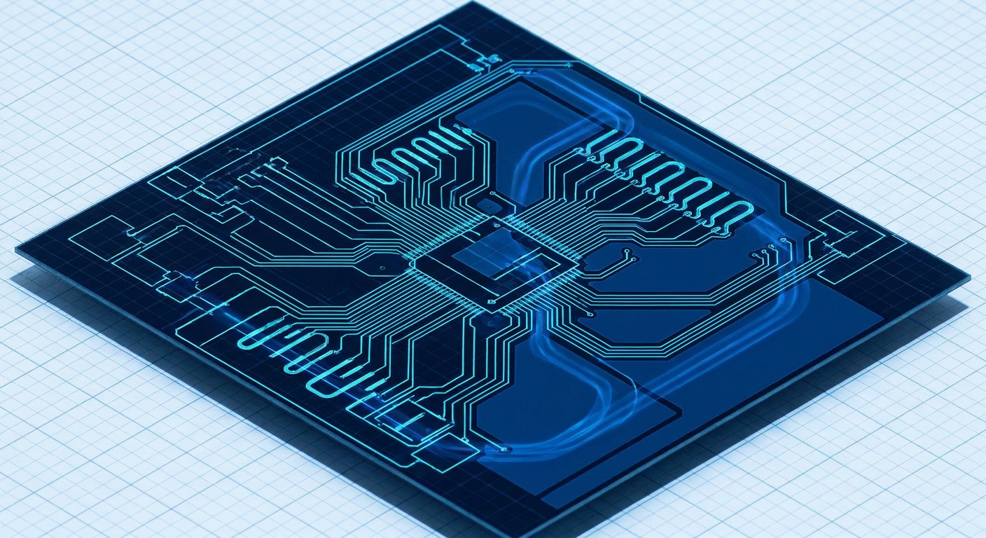
A clean Design Rule Check report in your EDA tool feels like the finish line. Every net connects, clearances stay above six mils, annular rings satisfy your fab house, and unrouted net counters drop to zero. Modern reinforcement learning PCB routers like Quilter and DeepPCB now hit these geometric targets in minutes, solving complex multi-layer boards that would take a human layout engineer days to untangle.
Then the first batch of prototypes arrives from assembly. The board powers up, but the USB 3.0 transceiver drops packets, an SPI flash bus corrupts at 40 MHz, and radiated emissions test results fail Class B compliance by 14 dB. When you probe the board with a high-bandwidth oscilloscope, you do not find shorts or opens. You find severe ringing, ground bounce, and phase skew.
For a solo hardware engineer at an early-stage startup, this failure mode is fatal to project schedules. A respin does not just cost $1,500 in bare boards and SMT setup fees. It burns three weeks of waiting, ties up capital, and stalls firmware bring-up. The root cause is not an undetected short circuit. The fundamental problem is that geometric clearance checking has almost nothing to do with signal integrity, electromagnetic fields, or return paths.
The Geometry Trap in Traditional and AI Routing
Design Rule Checks exist to enforce manufacturing limits, not physics. When Altium, KiCad, or an AI routing backend runs DRC, it validates planar boundaries. It measures whether copper trace A is at least 0.15 mm away from trace B. It verifies that drill diameters fit within annular pads. It confirms that solder mask expansions prevent bridged pins.
+-------------------------------------------------------------+
|                   WHAT EDA DRC VALIDATES                    |
|  [x] Minimum trace width (e.g., 0.127 mm)                   |
|  [x] Copper-to-copper clearance (e.g., 0.15 mm)             |
|  [x] Annular ring breakout and hole size                    |
|  [x] Netlist topological connectivity (Point A to Point B)  |
+-------------------------------------------------------------+
|                 WHAT EDA DRC ROUTINELY IGNORES              |
|  [ ] Return current reference plane continuity              |
|  [ ] High-frequency loop inductance area                    |
|  [ ] Reference plane swapping without stitching vias        |
|  [ ] Parasitic capacitive loading from unintended stubs     |
|  [ ] Dynamic impedance changes across split power planes    |
+-------------------------------------------------------------+
Reinforcement learning models optimize reward functions. In current commercial implementations, the reward functions heavily prioritize topological completion: connecting 100% of nets without physical collisions while respecting clearance boundaries. Some engines incorporate basic length-matching metrics or rudimentary single-ended impedance target widths based on user-supplied stackups.
However, high-frequency signals do not travel solely inside copper traces. They travel in the dielectric space between the trace and its nearest reference plane as electromagnetic waves. The signal current on the trace requires an equal and opposite return current directly underneath it. If an algorithm routes a signal over a plane split, or transitions a trace from layer 1 to layer 4 without providing a nearby ground return via, the return current detours. DRC marks the net as 100% routed, but the electrical circuit now possesses a massive inductive loop.
Anatomy of an Invisible Return Path Failure
To understand why reinforcement learning engines struggle with return currents, consider a four-layer stackup: Signal 1, Ground Plane 2, Power Plane 3, and Signal 2. This is the standard stackup for budget-conscious IoT products.
When a 50-ohm single-ended trace runs along Signal 1, its return current travels on Ground Plane 2, directly beneath the trace. The loop area between signal and return is microscopic, maintaining tight characteristic impedance and minimal electromagnetic radiation.
When an automated router encounters congestion on Signal 1, it places a via, drops the trace down to Signal 2, and continues routing. To the DRC engine, this connection is valid. The netlist is satisfied.
To the signal current, the reference plane on Signal 2 is Power Plane 3, not Ground Plane 2. The return current cannot jump from Plane 2 to Plane 3 through the dielectric without significant impedance. The return current must wander across the board until it finds a decoupling capacitor or an edge-stitching via that connects Plane 2 and Plane 3.
  Signal Trace (Layer 1) --------+ (Via)
                                 |
  GND Plane (Layer 2)            |     [Return current must detour]
  =======================        |
  PWR Plane (Layer 3)            |
  =======================        |     [Large Loop = EMI Spikes]
                                 +--------> Signal Trace (Layer 4)
The consequences of this detour are immediate:
- Inductance Spikes: The loop area expands by orders of magnitude. The characteristic impedance at the via transition spikes from 50 ohms to over 120 ohms, creating reflections that degrade digital rise times.
- Severe Crosstalk: Detouring return currents share copper with adjacent signal returns, inducing ground bounce and jitter into unrelated analog or digital lines.
- Radiation: The enlarged loop functions as an efficient slot antenna. During EMC testing, this loop radiates energy at harmonics of the clock frequency, blowing past regulatory thresholds.
Because traditional DRC engines do not trace closed loop areas for dynamic return currents, this design passes automated verification without a single warning.
Differential Pairs and Pseudo-Symmetry
A common misconception among junior engineers is that differential pairs, such as USB D+/D- or Ethernet TX+/TX-, do not require a ground reference plane because the return current flows through the opposing trace. This is only true if the traces are perfectly coupled and driven with zero common-mode noise, a condition that never happens in practice.
In reality, differential microstrips on high-speed boards still couple strongly to the reference plane directly underneath them. When an AI router treats a differential pair as merely two coupled lines that must maintain a specific spacing, it often performs asymmetric via drops or snakes one line around a mounting hole while the other stays straight.
The Phase Skew Problem
When trace lengths differ by even a fraction of a millimeter at gigabit speeds, or when one trace switches layers two millimeters before its pair, the differential signal converts into a common-mode signal. Common-mode currents do not cancel each other out. They radiate directly into the environment and distort the differential receiver's eye diagram.
Reinforcement learning models trained on visual PCB images or graph networks often generate serpentine delay lines to fix total length discrepancies. However, placing delay compensation at the very end of a trace rather than immediately at the point of divergence leaves the common-mode discontinuity unmitigated across the rest of the board.
Illustrative Routing Benchmark: AI Engines vs Traditional SI Constraints
To visualize how different routing engines handle high-speed constraints on a typical 4-layer microcontroller development board, consider this representative benchmark. The board features an STM32 running an 80 MHz external memory interface, a USB 2.0 High-Speed link (480 Mbps), and two high-speed SPI channels.
Receipts Block: Illustrative Composite Comparison based on standard benchmark test cases across modern routing tools on a 4-layer FR4 stackup (1.6 mm thickness, 1 oz copper).
| Metric / Constraint | Altium Situs (Traditional Heuristic) | DeepPCB (Reinforcement Learning) | Quilter AI (Physics/RL Hybrid) | Experienced Layout Engineer (Manual) |
|---|---|---|---|---|
| Completion Rate (100% Target) | 91.4% (Stalls on dense BGA) | 100.0% (Completed in 4 min) | 100.0% (Completed in 12 min) | 100.0% (Manual 14 hours) |
| DRC Violations Reported | 0 on routed nets (8 unrouted) | 0 violations | 0 violations | 0 violations |
| Reference Plane Splits Crossed | 14 unmitigated splits | 9 unmitigated splits | 2 unmitigated splits | 0 splits crossed |
| Via Transitions Without GND Return Via | 22 layer jumps | 18 layer jumps | 4 layer jumps | 0 layer jumps |
| USB 2.0 Eye Diagram Margin (Simulated) | Failed (Unrouted) | 8% eye mask margin | 24% eye mask margin | 42% eye mask margin |
| Radiated EMI at 480 MHz Harmonic | Untestable | +8 dB over FCC Class B | -3 dB below FCC Class B | -11 dB below FCC Class B |
Traditional heuristic routers fail primarily on completion. They give up when routing density increases, forcing the engineer to finish manually.
Pure reinforcement learning engines achieve 100% completion by treating empty copper layers as free real estate. They jump across layers freely, dropping vias wherever clearance allows. The resulting board passes DRC, but the electrical performance degrades significantly due to unstitched return transitions.
Newer physics-guided AI engines show substantial improvements by penalizing layer jumps that lack adjacent ground continuity. Yet, even with these advances, automated tools cannot replace domain knowledge when handling mixed-signal partitioning, crystal oscillator keeps, and sensitive switching converter return loops.
Thermal Traps and Power Delivery Blindspots
Signal integrity issues grab the most attention, but power integrity and thermal management suffer from the same geometric blindness. Automated routers are notorious for creating swiss-cheese ground planes.
When an AI router drops a cluster of vias under a dense micro-controller or power management IC (PMIC), it frequently places the drill holes close together. While each via adheres to standard hole-to-hole clearance rules, the overlapping anti-pads on internal ground layers effectively sever the copper plane.
  Ground Plane Copper (Solid)
  ###############################################
  ###########    (Via)       (Via)    ###########
  ########     [Anti-Pad]  [Anti-Pad]    ########
  ######                                   ######  <-- Severed Neck
  ########     [Anti-Pad]  [Anti-Pad]    ########      High DC Resistance
  ###########    (Via)       (Via)    ###########
  ###############################################
This creates two severe problems:
- Thermal Bottlenecks: Modern power packages, such as QFNs with exposed thermal pads, depend on continuous copper pours and unbroken via stitching to sink heat into internal planes. Severed planes trap heat at the component package, pushing junction temperatures beyond safe operating margins.
- DC IR Drop: A return current carrying 3 amps from a buck converter output back to its ground terminal might be forced through a narrow 10-mil sliver of copper between via anti-pads. The resulting voltage drop disrupts power rail regulation and creates localized hot spots on the PCB.
Automated DRC tools will not flag a copper sliver as long as it meets minimum trace width specifications. They do not calculate current density or thermal dissipation unless you feed the design into an expensive, dedicated multiphysics solver.
The Solo Engineer's Pre- and Post-Routing Audit Checklist
If you use AI autorouters or automated layout tools to accelerate your design cycle, you must treat their output as a rough draft rather than production-ready Gerber files. Relying on an automated DRC pass before sending files to a fab like JLCPCB, PCBWay, or Eurocircuits is a recipe for expensive respins.
Use this systematic checklist before handing nets to an algorithm and after receiving the generated layout.
Phase 1: Pre-Routing Setup and Net Pinning
- Pin Critical Nets to Manual Layout: Never let an autorouter touch the switching loop of a DC-DC converter, the crystal oscillator lines, the sensitive RF front-end, or high-speed differential pairs (USB, PCIe, Ethernet). Route these by hand first, verify their return paths, and lock their positions.
- Define Strict Keepout Zones: Draw keepout regions on internal layers under analog signal traces and crystal oscillators to prevent the autorouter from running noisy digital lines directly underneath sensitive nodes.
- Enforce Differential Pair Rules in EDA: Set tight intra-pair length matching tolerances (within 0.1 mm) and maximum uncoupled length limits in your design rules prior to running automated layout.
Phase 2: Post-Routing Return Path Audit
- Track Every Layer Transition on High-Speed Lines: For every via on a signal line running faster than 25 MHz, verify that an adjacent ground return via exists within 1.0 mm. If the trace transitions between planes of different potentials (e.g., Ground to Power), place a 0.1 uF stitching capacitor immediately next to the transition.
- Inspect Internal Planes in 2D Visual Mode: Turn off all trace layers and inspect your ground planes individually. Look for clusters of via anti-pads that create copper bottlenecks, slots, or isolated islands.
- Verify Switching Converter Return Loops: Check that the ground pads of your buck/boost input capacitors, output capacitors, and IC ground pins connect through wide, uninterrupted copper pours on Layer 1 before connecting to internal planes.
- Audit Thermal Reliefs on High-Current Paths: Ensure that high-current inductors and power MOSFET pads use solid connections rather than thermal relief spokes where heat extraction and low impedance are paramount.
What This Means for IntelCAD
Building modern hardware requires tools that understand electromagnetic and thermal physics, not just geometric clearance grids. The mission at IntelCAD (intelcad.ai) is to build automated layout and co-pilot systems that treat return paths, layer transitions, and live BOM supply chain constraints as primary physical variables rather than downstream afterthoughts.
A board that passes geometric DRC but fails signal integrity is an unmanufacturable design. Bridging schematic capture, physical stackup analysis, and component sourcing into a unified, physics-aware workflow is the only way to make automated PCB design truly production-ready.
Direct Answer: Why AI Routers Fail at Signal Integrity
AI autorouters pass Design Rule Checks while failing signal integrity because DRC only measures physical distances and topological connectivity. DRC engines confirm that a net connects Point A to Point B without violating planar spacing clearances, but they do not calculate dynamic loop inductance, high-frequency return current detours across split reference planes, or phase skew across asymmetric vias. High-speed signals depend on electromagnetic fields that travel through dielectric space and reference planes; because standard routing algorithms optimize for net completion rather than field behavior, a DRC-clean board can easily fail EMC testing and high-speed data transmission.
Moving from Push-Button Hype to Production Reality
Automated routing has made impressive progress over the past two years. Reinforcement learning algorithms can now untangle complex interconnects that would exhaust human patience. However, treating these tools as magical push-button solutions ignores the underlying physics of electrical circuits.
For solo engineers and hardware founders, the real risk is not taking three days to route a board. The real risk is burning four weeks and thousands of dollars on a respin because a DRC-clean board was electrically non-functional. Treat automated layout engines as powerful draft assistants: let them route non-critical digital logic and control lines, but keep your hands on the critical paths, inspect your reference planes with care, and never trust a zero-error DRC report without auditing where the return current flows.
Sources
- Quilter AI: PCB Autorouting in 2026: A Review of Traditional Tools vs. Quilter's AI Approach, https://www.quilter.ai/blog/pcb-autorouting-in-2026-a-review-of-traditional-tools-vs-quilters-ai-approach
- Quilter AI: Why New Routing Problems Keep Breaking Old Tools, https://www.quilter.ai/blog/new-routing-breaking-old-tools
- DeepPCB: The Autorouter Broke Your Trust. Here's What's Actually Different Now, https://deeppcb.ai/the-autorouter-broke-your-trust-heres-whats-actually-different-now/
- JLCPCB: Can PCB Autorouters Really Deliver Production-Ready Designs?, https://jlcpcb.com/blog/pcb-autorouter-production
- Sierra Circuits: 8 Factors that Lead to Signal Integrity Issues in a PCB, https://www.protoexpress.com/blog/signal-integrity-issues-in-pcb/
- Cadence: Signal Integrity Basics and Fundamentals in PCB Layout, https://resources.pcb.cadence.com/blog/2024-signal-integrity-basic
- Ansys / Synopsys: What is Signal Integrity?, https://ansys.synopsys.com/simulation-topics/what-is-signal-integrity