The open-source release of Newton, an NVIDIA Warp-based physics simulation engine integrating MuJoCo-Warp, alongside the rollout of Genesis World 1.0, marks a distinct operational shift for mechanism designers. For decades, roboticists and mechanical engineers evaluated linkages, robot arms, and multi-body assemblies using standard kinematic solvers. Those tools assume a clean mathematical world: zero-friction revolute joints, infinitely stiff prismatic rails, and instantaneous velocity changes without dynamic stick-slip.
When those idealized designs move from a CAD display to 5-axis CNC machining centers, the physical hardware tells a different story. Off-axis loads twist precision bronze bushings, causing them to bind. Stick-slip friction at low speeds forces position servos into hunting oscillations. Cable drives experience capstan friction losses that deplete motor torque margins. By the time a physical prototype binds on the test bench, thousands of dollars in wire EDM runs, machined 7075-T6 aluminum billets, and custom ground shafts are already wasted.
GPU-accelerated physics engines bring high-speed dynamic contact, anisotropic friction, and non-linear joint compliance into early mechanism design. Instead of running kinematics as an isolated geometric exercise, engineers can now simulate millions of dynamic contact timesteps in seconds. Catching joint binding, motor stall, and thermal-expansion interference before releasing production drawings changes how small robotics shops and mechanism design teams allocate their build budgets.
The Frictionless Lie of Standard Kinematics
Standard kinematic software treats joints as algebraic constraints. If you define a revolute joint in standard CAD software or a basic forward/inverse kinematics package, the solver treats the degree of freedom as a pure rotation around a single vector. The joint has no mass, no clearance, no surface roughness, and no resistance to motion unless an arbitrary damping coefficient is added to the joint property sheet.
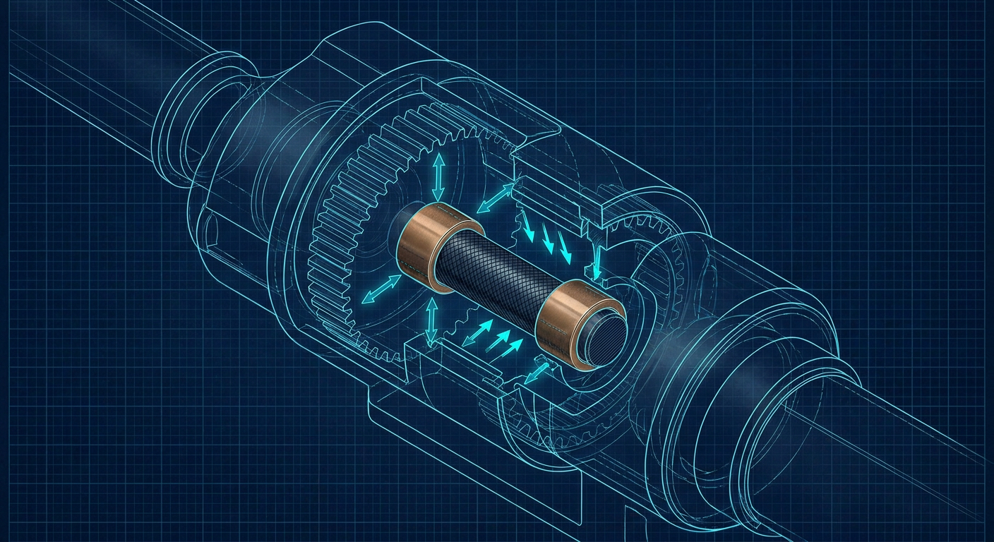
On the shop floor, a joint is not a line in space. It is a pair of mating surfaces separated by a grease film, a dry PTFE liner, or a set of bearing balls riding on ground raceways. Every real joint presents three distinct frictional challenges that static kinematic tools ignore:
- Static vs Kinetic Breakaway (Stick-Slip): A joint requires higher torque to start moving than to keep moving. In low-speed, high-precision positioning mechanisms, this difference causes the motor to wind up, snap forward, overshoot the target, and oscillate.
- Load-Dependent Normal Forces: When an overhung payload creates an off-axis moment, the normal forces inside a pin bushing spike dramatically at the outer edges. This edge-loading increases Coulomb friction far beyond nominal radial load assumptions.
- Clearance Tilting and Wedging: Standard kinematic tools assume parts remain perfectly coaxial. In reality, an H7/g6 running fit permits microscopic angular deflection. Under dynamic acceleration, that angular tilt can cause the pin to wedge against the bore corners, causing mechanical seizure.
When a mechanism engineer sizes a motor based on frictionless inverse dynamics, they calculate torque purely from inertial acceleration ($J \cdot \alpha$) and gravitational load ($ au_g$). On a 4-axis pick-and-place linkage moving at 2 m/s, friction and edge-loading can easily add 30 to 50 percent to the required peak torque. If the motor lacks sufficient thermal headroom, it will saturate current limits, fault out on drive errors, or overheat within minutes of continuous cycle testing.
How GPU Physics Solvers Change Dynamic Verification
Until recently, running dynamic contact simulation with non-linear friction meant setting up complex finite element analysis (FEA) runs in packages like Abaqus or ANSYS, or waiting hours for transient multi-body dynamics solvers to converge on CPU cores. These tools are far too slow for iterative mechanism synthesis, where link lengths, pivot offsets, and bushing diameters change multiple times per day.
Physics engines like Newton and Genesis use GPU parallelism to calculate dynamic contact and multi-body constraints at thousands of frames per second. Newton runs atop NVIDIA Warp, executing low-level spatial algebra and contact dynamics directly on CUDA cores. Genesis unifies multi-physics solvers, enabling simultaneous evaluation of rigid linkages, compliant cables, and localized contact friction.
Traditional Kinematics Pipeline:
[CAD Geometry] -> [Ideal Mate Constraints] -> [Geometric IK Solver] -> [Machining]
                                                                         |
                                              Result: Unmodeled binding on bench

GPU-Accelerated Dynamic Pipeline:
[CAD Geometry] -> [Clearance & Surface Def] -> [Newton / Genesis Solver] -> [Verified CAD]
                                                       |
                                  Evaluates: Edge loads, stick-slip,
                                             capstan friction, thermal fits
Because these solvers execute thousands of parallel rollouts across varying payload weights, acceleration profiles, and friction coefficients ($\mu$), engineers can run Monte Carlo sweeps across real manufacturing tolerance bands before finalizing a bill of materials.
Simulating Real-World Friction Mechanisms
Newton includes explicit contact and friction routines designed to capture complex transmission behaviors, such as tendon-pulley capstan friction and pinhole binding. In a cable-driven manipulator, friction along a curved sheath or capstan drum does not follow simple linear damping. It follows the Euler-Eytelwein capstan equation:
$$T_{\text{load}} = T_{\text{hold}} \cdot e^{\mu \theta}$$
Where $\mu$ is the friction coefficient and $\theta$ is the total wrap angle in radians. A slight accumulation of wrap angle through a 3D-routed cable guide can turn a smooth cable drive into a high-friction brake. By evaluating these non-linear equations within dynamic GPU rollouts, engineers can identify where routing paths must be modified to prevent line binding.
Similarly, when simulating revolute joints with realistic clearances, GPU solvers handle non-smooth contact mechanics. When an arm decelerates rapidly, the solver calculates the exact point where the pin strikes the bushing wall, resolving the normal force, the resulting frictional traction, and the transient deceleration spike.
The Cost of Shop Floor Surprises
To understand why high-fidelity dynamic physics matters to an engineering budget, consider a standard four-bar parallel lift mechanism built for an automated logistics cell. The engineering team designs the linkages in CAD, verifies clearance envelopes using kinematic motion analysis, and selects brushless DC (BLDC) motors paired with 50:1 planetary gearboxes based on inertial torque calculations.
The prototype requires four custom-machined 6061-T6 aluminum link arms, ground 17-4 PH stainless steel pivot pins, and SAE 841 oil-impregnated bronze bushings.
Illustrative Friction and Torque Discrepancy
The following table represents an illustrative composite of a typical high-acceleration linkage evaluation, comparing standard frictionless kinematic predictions against GPU dynamic physics and physical dynamometer shop-floor testing.
| Evaluation Metric | Frictionless CAD Kinematics | GPU Dynamic Physics (Newton) | Physical Bench Test (Shop Prototype) | Error vs Reality (CAD) | Error vs Reality (GPU) | | :--- | :--- | :--- | :--- | :--- | :--- | | | Peak Joint Breakaway Torque | 0.00 N-m (Assumed zero) | 3.85 N-m | 4.10 N-m | -100.0% | -6.1% | | Continuous Joint Friction Loss | 0.20 N-m (Linear viscous) | 1.95 N-m (Coulomb + Stribeck) | 2.10 N-m | -90.5% | -7.1% | | Max Motor Drive Current | 12.4 A | 18.2 A | 19.1 A | -35.1% | -4.7% | | Bushing Edge-Load Reaction | Uncalculated | 420 N | 465 N | N/A | -9.7% | | Cycle Settlement Time (to 50µm)| 120 ms | 245 ms | 260 ms | -53.8% | -5.7% |
Note: Composite illustrative data representing a 4-bar linkage (5 kg payload, 1.5 m/s peak velocity, 2.5 g acceleration, SAE 841 bronze on steel pin with 0.025 mm clearance).
When this mechanism is built without dynamic friction verification, the consequences are immediate:
- Motor Thermal Saturation: The motor controller draws 19.1 A during acceleration instead of the calculated 12.4 A. In continuous cycling, the motor windings exceed their 130°C thermal limit within eight minutes, tripping the driver.
- Settling Time Penalties: The kinematic model predicted a 120 ms settling time. Because static friction creates stick-slip near zero velocity, the position loop takes 260 ms to settle within tolerance, cutting machine throughput in half.
- Scrapped Parts: To resolve the binding, the shop must either bore out the link arm housings to fit larger needle roller bearings (costing $800 in rework and two days of machine time) or scrap the motor-gearbox assemblies and purchase larger units with higher peak torque ratings, adding weeks of lead time.
Practical Framework: Setting Up Dynamic Contact Checks
Mechanism designers do not need to simulate every bolt thread or dowel pin. However, applying GPU physics engines to critical kinematic chains before committing to production requires a structured workflow. Here is a decision frame for evaluating mechanisms in Newton or Genesis.
Dynamic Verification Checklist:

1. Identify Critical Pivot Pairs
   [ ] Classify high-load joints (sliding vs rolling contact)
   [ ] Identify overhung moments causing edge-loading

2. Define Physical Friction Parameters
   [ ] Static friction coefficient (µs)
   [ ] Kinetic / dynamic friction coefficient (µk)
   [ ] Radial and axial clearance bounds (e.g., ISO H7/g6 or H7/h6)

3. Execute Dynamic Multi-Rate Simulation
   [ ] Run motion profile at 100%, 125%, and 150% target velocity
   [ ] Apply load reversal step inputs to evaluate stick-slip
   [ ] Measure torque margin against motor continuous curves

4. Modify Mechanism Parameters
   [ ] Widen bearing stance to reduce moment-induced normal loads
   [ ] Transition sliding bushings to needle rollers if friction > 15% budget
   [ ] Update motor selection with verified RMS current profiles
Step 1: Characterize Joint Interfaces Accurately
Never use default friction coefficients from generic software libraries. Group mechanism interfaces by their real-world contact conditions:
- Dry Polymer on Anodized Aluminum (e.g., Igus iglidur on hardcoat aluminum): $\mu_s \approx 0.25 - 0.35$, $\mu_k \approx 0.15 - 0.22$.
- Sintered Bronze on Ground Steel (SAE 841, ISO VG 68 oil): $\mu_s \approx 0.12 - 0.18$, $\mu_k \approx 0.08 - 0.12$.
- Hardened Steel Ball Bearings: Effective friction is low ($\mu \approx 0.0015 - 0.003$), but pre-load drag torque and seal drag must be added as a constant opposing torque.
Step 2: Model Geometric Clearances and Asymmetric Stances
One common cause of mechanical binding is an insufficient bearing stance. If a sliding carriage rides on two parallel linear shafts, the distance between the bushings along the shaft ($L$) must be sufficiently large relative to the span between the shafts ($W$).
According to the classic 2:1 rule of thumb for linear bearings, if $W / L > 2$, the carriage will experience binding under off-center driving forces. A GPU physics engine directly reveals this failure mode: as you shift the simulated actuator attachment point away from the center of mass, the contact normal forces on the opposing bushings spike asymptotically, stalling the drive in the simulation before the rail is ever bolted to an aluminum tooling plate.
Step 3: Check Torque Curves Against Thermal RMS Limits
Peak torque gets a mechanism moving, but root-mean-square (RMS) torque determines whether the motor burns out. The dynamic simulation exports a continuous torque timeline $\tau(t)$ over a complete machine cycle period $T$:
$$T_{\text{RMS}} = \sqrt{\frac{1}{T} \int_{0}^{T} \tau(t)^2 , dt}$$
If $T_{\text{RMS}}$ exceeds the motor manufacturer's continuous rated torque at operating temperature, the mechanism is under-actuated. Friction-aware simulation captures the parasitic drag that inflates this integral during constant-speed cruise segments, preventing undersized motor selection.
What This Means for Mexaio AI
Generative design cannot stop at producing static, organic shapes that look impressive in a CAD viewport. In robotics and high-speed automation, geometry is meaningless if the resulting joints seize under real-world dynamic loads or require impossible machining tolerances to operate smoothly.
Tools like Mexaio AI approach mechanical design by generating fully parametric, editable kinematic assemblies where linkage geometry, pivot centers, and structural clearances are directly tied to dynamic performance. By integrating physics-aware simulation early in the generative loop, the software ensures that generated mechanisms account for joint friction, motor torque limits, and realistic bearing tolerances. Instead of outputting dead meshes that require manual remodeling and guess-and-check motor sizing, the system produces manufacture-ready CAD models verified against dynamic physical constraints.
Preparing the Shop for Physics-Driven Design
Mechanism engineering is moving away from the era of isolated CAD drawings and post-machining troubleshooting. The availability of open-source GPU engines like Newton and platform ecosystems like Genesis allows even small engineering shops to run physics simulations that were once restricted to high-budget aerospace labs.
Moving forward, mechanical designers should take concrete steps to modernize their verification workflow:
- Audit Existing Kinematic Models: Review current robotic sub-assemblies that experience mysterious motor overheating or tracking errors. Re-run their trajectories through a dynamic contact solver with realistic Coulomb friction coefficients.
- Incorporate Clearance Tolerances into Sim Models: Do not model pivot pins with nominal line-to-line contact. Introduce ISO fit clearances (such as H7/h6 or H7/f7) to observe how pin tilting and dynamic edge-loading affect driving torque.
- Bridge the CAD-to-Physics Gap: Build automated pipelines that export mechanism URDFs or OpenUSD models directly into Newton or Warp environments to verify motor margins before cutting metal on the shop floor.
Simulating joint friction before releasing purchase orders for CNC machining and precision actuators is no longer a luxury. It is the most reliable way to ensure that the parts arriving from the machine shop assemble cleanly, move smoothly, and hit their cycle targets on the very first power-up.
Sources
- NVIDIA Developer Blog: Announcing Newton, an Open-Source Physics Engine for Robotics Simulation: https://developer.nvidia.com/blog/announcing-newton-an-open-source-physics-engine-for-robotics-simulation/
- GitHub Repository: Newton GPU-Accelerated Physics Simulation: https://github.com/newton-physics/newton
- Genesis AI Research: The Role of Simulation in Scalable Robotics and Genesis World 1.0: https://www.genesis.ai/blog/the-role-of-simulation-in-scalable-robotics-genesis-world-10-and-the-path-forward
- CoppeliaSim Manual: Contact and Friction Characteristics Across Dynamic Engines: https://manual.coppeliarobotics.com/en/physicsEngineDifferences.htm
- MATLAB Simulink: Inverse Kinematics and Dynamic Motion Profiling: https://www.mathworks.com/discovery/inverse-kinematics.html