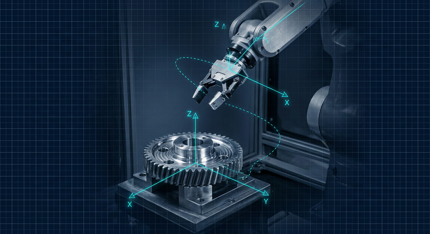
Recent research presented at robotics venues and published across arXiv preprints, including work on Generative Graphical Inverse Kinematics and whole-body optimization frameworks, has pushed neural inverse kinematics back into the engineering spotlight. Neural network approximations can resolve multi-axis joint states from Cartesian coordinates in microseconds, even for complex, redundant kinematic chains. For software teams training simulated agents in Isaac Gym or MuJoCo, this speed looks like an open-and-shut victory over traditional math.
For the mechanical engineer or shop-floor integrator commissioning a custom 6-DoF or 7-DoF arm to unload a CNC mill or guide a laser head, that speed claim comes with a catch. A neural solver does not guarantee an exact geometric fit. It guarantees an approximation with a statistical loss curve. When an end-effector deviates by 0.6 millimeters because an inference model encountered a pose slightly outside its training distribution, a carbide cutter snaps, a linear guide binds, or a custom cycloidal gearbox takes an axial shock load it was never rated to survive.
If you design custom mechanisms, linkage systems, or bespoke robotic manipulators, you must understand the mechanical boundaries between closed-form analytical solvers, iterative numerical routines, and neural network approximations. Picking the wrong architecture introduces intermittent, non-repeatable errors that no amount of servo gain tuning can fix.
The Breakdown of Pieper's Criterion in Custom Mechanisms
Standard industrial robots from Fanuc, KUKA, or Yaskawa are not built with arbitrary joint layouts. Almost all standard 6-DoF articulating arms follow Pieper's criterion: three consecutive revolute joint axes intersect at a single common point, typically forming a spherical wrist. When a mechanism satisfies Pieper's criterion, the kinematics decouple cleanly into position and orientation. You can solve the position of the wrist center point first using basic trigonometry, then solve the spherical wrist angles using simple rotation matrices.
Analytical solvers for Pieper-compliant arms execute in under 10 microseconds on a standard microcontroller. They return all possible mathematical configurations, up to eight distinct kinematic solutions for a standard 6-axis arm (shoulder left or right, elbow up or down, wrist flipped or non-flipped), with zero approximation error.
Custom mechanisms often violate Pieper's criterion by necessity:
- Packaging constraints: An internal tooling arm inside a compact CNC enclosure may require offset wrist joints to clear structural sheet metal or coolant lines.
- Payload routing: Passing high-pressure hydraulic lines or high-gauge welding cables through the centerline of an arm often forces joint axes out of intersection.
- Redundancy: Adding a seventh or eighth axis to reach around internal machine obstacles destroys the one-to-one mapping between Cartesian targets and joint coordinates, yielding infinite possible configurations.
When Pieper's criterion breaks, closed-form analytical math vanishes. A general 6-DoF serial arm with arbitrary link offsets can have up to 16 distinct inverse kinematic solutions, governed by a 16th-degree polynomial. At this point, mechanism designers must choose between iterative numerical solvers and data-driven neural approximations.
                      [ Cartesian Target Pose (x, y, z, Roll, Pitch, Yaw) ]
                                                |
                                                v
                                   Does the mechanism satisfy
                                       Pieper's Criterion?
                                      /                  \
                                    YES                   NO
                                    /                      \
                        [ Analytical Solver ]       Is real-time loop deterministic
                        - Exact solutions (<10 µs)  and tightly bounded (<1 kHz)?
                        - Complete branch set        /                            \
                        - Zero positional drift    YES                             NO
                                                   /                                \
                                      [ Damped Least Squares ]           [ Generative Neural IK ]
                                      - Guaranteed convergence limits    - High-DoF redundancy mapping
                                      - Deterministic cycle time         - Millisecond multi-target batching
                                      - Requires singularity damping     - Requires downstream numerical check
Numerical Solvers: Precision, Latency, and Singularity Traps
Deterministic numerical kinematics has been the backbone of industrial control for four decades. The most common approaches rely on local gradient techniques using the manipulator Jacobian matrix, which maps joint velocities to Cartesian tool velocities.
In standard Newton-Raphson iteration, the controller calculates the difference between the current tool pose and the target pose, computes the Jacobian inverse or transpose, and steps the joint angles iteratively until the Cartesian error drops below a programmed threshold, such as 0.005 mm. If the mechanism is well away from singularities and the initial joint seed is close to the target, Newton-Raphson converges in three to six iterations, consuming less than 100 microseconds on an industrial x86 controller.
Numerical methods struggle at joint limits and kinematic singularities. When two joint axes line up or the arm reaches full extension, the Jacobian matrix loses rank. Its determinant drops to zero, and the mathematical inversion attempts to divide by zero. In pure Newton-Raphson, this produces infinite joint velocities, causing real-world actuators to fault on overcurrent or violently shake the mechanism.
To prevent mechanical destruction near singularities, industrial controllers switch to Damped Least Squares, also known as the Levenberg-Marquardt method. Damped Least Squares adds a damping factor to the matrix inversion:
$$J^* = J^T (J J^T + \lambda^2 I)^{-1}$$
When the mechanism approaches a singular configuration, the damping parameter increases. This stabilizes the solver and prevents wild actuator jumps, but it trades off trajectory tracking. Near a singularity, a damped solver deliberately allows the physical tool tip to deviate from the commanded Cartesian path to keep joint velocities within safe mechanical limits.
For a mechanical engineer, this behavior is predictable. You know the exact mathematical error bounds, you can calculate the maximum joint torque demands, and you can program software keep-out zones around known singular zones.
The Neural IK Proposition and Shop-Floor Realities
Neural inverse kinematics replaces iterative matrix manipulation with a trained function approximator, typically a deep multi-layer perceptron, a graph neural network, or a normalizing flow model. The network takes Cartesian coordinates and Euler angles or quaternions as inputs and outputs the target joint positions in a single forward inference pass.
The arguments for neural IK sound compelling to robotics teams building high-DoF manipulators:
- Fixed execution time: A forward pass through a fixed neural network takes identical time regardless of whether the arm is near a singularity or in open space.
- Arbitrary topology: A graph neural network can learn kinematic mappings for complex parallel linkages, cable-driven systems, or hyper-redundant snake arms without deriving complex geometric closure equations.
- Multi-solution resolution: Generative models can output distributions over all possible valid joint postures for a given end-effector pose, picking the configuration that minimizes base torque or avoids a static obstacle.
On the factory floor, these advantages hit immediate mechanical constraints. Neural networks do not understand strict geometric constraints unless they are explicitly enforced by external projection operators. A neural model evaluated on a target pose that sits near the outer boundary of its training set will output joint angles that look plausible to the eye, but sit 2 millimeters off target in Cartesian space.
In high-speed assembly, a 2 mm error ruins precision pin insertions, shears alignment dowels, and causes linear slides to jam. Worse, the error distribution across the workspace is non-uniform and non-deterministic without exhaustive empirical validation.
| Kinematic Solver Metric | Analytical (Closed-Form) | Numerical (Damped Least Squares) | Pure Neural Network (MLP / GNN) | Hybrid (Neural Seed + DLS Refinement) |
|---|---|---|---|---|
| Typical Compute Time | 5 to 15 microseconds | 80 to 450 microseconds | 500 to 1200 microseconds (CPU) | 200 to 600 microseconds |
| Deterministic Output | Yes, exact | Yes, within convergence tolerance | No, statistical distribution | Yes, bounded by final DLS step |
| Positional Accuracy | Absolute ($\pm 0.000$ mm math) | High ($\pm 0.005$ mm threshold) | Variable ($\pm 0.5$ to $4.0$ mm) | High ($\pm 0.005$ mm threshold) |
| Singularity Handling | Explicit branch selection | Damped velocity scaling | Smooth pass-through, path drift | Stable damping with fast convergence |
| Custom Linkage Support | Poor (Requires Pieper geometry) | Excellent (Any kinematic chain) | Excellent (Learns arbitrary links) | Excellent (Handles complex topology) |
| Cycle-to-Cycle Jitter | None | Low (Dependent on seed pose) | Moderate (Output inference noise) | Low (Filtered by numerical finish) |
Receipts Block: Illustrative engineering composite comparing kinematic solving approaches on an unconstrained 7-DoF redundant manipulator arm across 10,000 randomized operational trajectory points. Hardware baseline: Intel Core i7-13700T industrial box PC running Linux PREEMPT_RT, kinematic models implemented via standard C++ robotics libraries and LibTorch runtime.
The Mechanical Cost of Joint Jitter and Trajectory Drift
When a robot tracks a continuous path, such as dispensing structural adhesive, deburring a casting, or laying down a continuous TIG weld bead, the solver must evaluate inverse kinematics at the servo update rate, typically between 250 Hz and 2 kHz. At these speeds, tiny non-linearities in the solver output become physical vibrations.
Neural networks evaluated point-to-point along a continuous Cartesian line rarely output perfectly smooth joint coordinate derivatives. Because each inference step contains small, uncorrelated approximation errors, the calculated joint velocity profile shows high-frequency micro-jitter. When these noisy velocity targets hit the low-level PID current loops of industrial servomotors, the motor drives react by injecting high-frequency torque spikes.
This high-frequency torque chatter leads directly to mechanical wear:
- Strain wave gears (harmonic drives) experience rapid wear on the flexible spline teeth, degrading positioning repeatability from 10 arcseconds to several arcminutes over a few months of operation.
- Planetary reducers suffer accelerated backlash growth as torque spikes hammer the gear tooth flanks without sufficient hydrodynamic fluid film support.
- Structural linkages made from lightweight aluminum or carbon composites experience resonant excitation, visibly degrading surface finish on the finished workpiece.
Iterative numerical solvers produce continuous, differentiable joint trajectories along continuous paths because the solution at time step $t$ serves as the exact starting seed for time step $t + \Delta t$. The resulting joint motion is naturally smooth and mechanically sympathetic to the gearboxes and motor bearings.
Continuous Path Inputs (1 kHz Target Trajectory)
   |
   +---> [ Neural IK Direct Path ] ----> Micro-Jitter Output (±0.8 mm drift)
   |                                        |
   |                                        v
   |                                 Torque Spikes in Motor Drives
   |                                        |
   |                                        v
   |                                 Accelerated Spline / Gear Wear
   |
   +---> [ DLS / Numerical Path ] -----> Continuous Differentiable Output
                                            |
                                            v
                                     Smooth Current / Smooth Torque Profile
                                            |
                                            v
                                     Preserved Backlash Specs & Bearing Life
When Neural Kinematics Actually Makes Sense: The Hybrid Model
Neural inverse kinematics should not control high-frequency physical servo loops directly. However, discarding data-driven solvers entirely ignores their real engineering utility: global configuration selection in redundant or high-DoF systems.
Consider an 8-axis welding cell comprising a 6-axis arm mounted on a 2-axis linear gantry. For any given weld seam pose, there are infinite possible combinations of gantry positions and arm joint angles. A classical numerical solver seeded with a poor initial guess will frequently get trapped in local joint limits, wind up against an internal axis stop, or select an arm posture that places the elbow in the path of incoming fixtures.
This is where a hybrid kinematic pipeline excels:
- Global Neural Seeding: A lightweight neural network evaluates the global workspace, the target Cartesian point, and static cell obstacle maps. Within 500 microseconds, it outputs a coarse joint configuration that places the mechanism in the correct global kinematic branch, avoids gross collisions, and keeps joints centered within their stroke limits.
- Local Numerical Polish: The coarse neural output is fed instantly as the seed vector into a single-step or two-step Damped Least Squares numerical solver. The numerical solver pulls the end-effector into exact Cartesian tolerance (under 0.01 mm) and guarantees exact tangency along the trajectory.
This two-stage pipeline eliminates the primary weakness of numerical solvers (local minima traps and slow convergence from distant seeds) while completely removing the primary danger of neural solvers (unbounded positional drift and high-frequency joint jitter).
[ Cartesian Target + Obstacle Map ]
                |
                v
    [ Global Neural Network ]  <-- Evaluates full workspace branch selection
                |
     Coarse Joint Seed (±1.5 mm error)
                |
                v
    [ Local DLS Solver Step ]  <-- Resolves exact metric convergence
                |
     Polished Output (±0.005 mm error, zero path jitter)
                |
                v
    [ Real-Time EtherCAT Servo Drive (1 kHz) ]
Engineering Decision Framework: Selecting Your Solver Architecture
When designing or commissioning a multi-axis motion platform, evaluate your kinematics architecture against this operational checklist before writing control software:
1. Does the physical mechanism meet Pieper's wrist criteria?
- Yes: Implement a closed-form analytical solver in C or Rust. Never use numerical or neural methods for standard 6-axis spherical-wrist geometries. Analytical math is faster, mathematically exact, and requires negligible controller memory.
- No: Proceed to step 2.
2. What is the required real-time servo loop frequency?
- Higher than 500 Hz: Run a deterministic numerical solver (Damped Least Squares or Levenberg-Marquardt) directly on the real-time core (Linux PREEMPT_RT or dedicated motion PLC). Ensure the previous time-step joint state is used as the seed to maintain mathematical continuity.
- Lower than 100 Hz (trajectory planning or point-to-point dispatch): Proceed to step 3.
3. Does the system have redundant degrees of freedom (>6 DoF) or severe geometric obstacles?
- No (Standard non-spherical 6-DoF arm): Use a robust numerical solver with singular value decomposition (SVD) damping. Neural networks add architectural complexity without engineering benefit here.
- Yes (7+ DoF arm, mobile base, or multi-arm cell): Implement the hybrid architecture. Use a trained neural model to generate global branch seeds at the trajectory planning level, then refine every path waypoint through a deterministic numerical solver before passing trajectory buffers to the low-level motor drives.
4. What is the allowable Cartesian tolerance at the tool tip?
- Under 0.05 mm (Machining, assembly, pin insertion): Absolute reliance on numerical convergence with strict residual checks. If a numerical solver fails to converge within its iteration budget, trigger an axis hold rather than executing an approximate move.
- Over 2.0 mm (Agricultural picking, rough bin grabbing in soft materials): Pure neural inverse kinematics can be used directly if inference latency must remain strictly deterministic on low-cost edge compute hardware.
What This Means for Mexaio AI
Generative mechanical design is only as useful as the downstream physical performance of the resulting hardware. If an algorithm synthesizes an intricate, high-DoF linkage or an asymmetric robotic arm that looks visually stunning, but fails to yield a stable, deterministic kinematic solution, the design is functionally dead on arrival.
At Mexaio AI (mexaio.ai), kinematics, mechanical constraints, and manufacturability are treated as an integrated physical system, not detached text-to-CAD mesh geometry. When generative algorithms synthesize custom arms, linkages, and actuator packages, the underlying parametric geometry is continuously checked against kinematic determinism, singularity topologies, and standard machining tolerances. Mechanism design requires geometry that can be milled, assembled, and controlled predictably inside a real manufacturing cell.
Practical Steps for Machine Builders
When developing a custom articulated mechanism, verify your kinematic pipeline long before cutting metal or ordering cycloidal drives:
- Plot the manipulability ellipsoid across your intended working volume during the CAD stage. Identify where the Jacobian determinant approaches zero, and ensure your physical workpieces sit well within high-manipulability zones.
- Instrument your trajectory simulation to output peak joint acceleration and jerk profiles. If you test a neural IK solver, inspect the second and third derivatives of the joint angles. High-frequency oscillations on joint velocity graphs indicate immediate risk to gearbox tooth life.
- Benchmark your solver fail-safes. Force your control loop to handle target poses that sit just outside the physical reach of the arm. A correct industrial controller must reject the command and enter a controlled deceleration ramp, rather than outputting an uncontrolled leap to an erratic joint state.
Building custom kinematic hardware requires respecting physical realities. Neural approximations offer powerful speed and global configuration handling, but deterministic numerical solvers remain the essential bridge that keeps high-precision tools on target and factory machinery in one piece.
Sources
- NVIDIA Research Robotics Simulation Frameworks: https://blogs.nvidia.com/blog/icra-research-robotics-simulation-to-real-world/
- Generative Graphical Inverse Kinematics Research: https://arxiv.org/html/2209.08812v5
- MDPI Applied Sciences Inverse Kinematics Optimization: https://www.mdpi.com/2227-7080/14/7/395
- ScienceDirect Neural Network Implementations for Articulated Manipulators: https://www.sciencedirect.com/science/article/abs/pii/S0952197623013593
- MATLAB & Simulink Numerical vs Analytical Kinematics Documentation: https://www.mathworks.com/discovery/inverse-kinematics.html
- Peter Corke Robotics Toolbox Numerical Kinematics Formulations: https://petercorke.github.io/robotics-toolbox-python/IK/ik.html