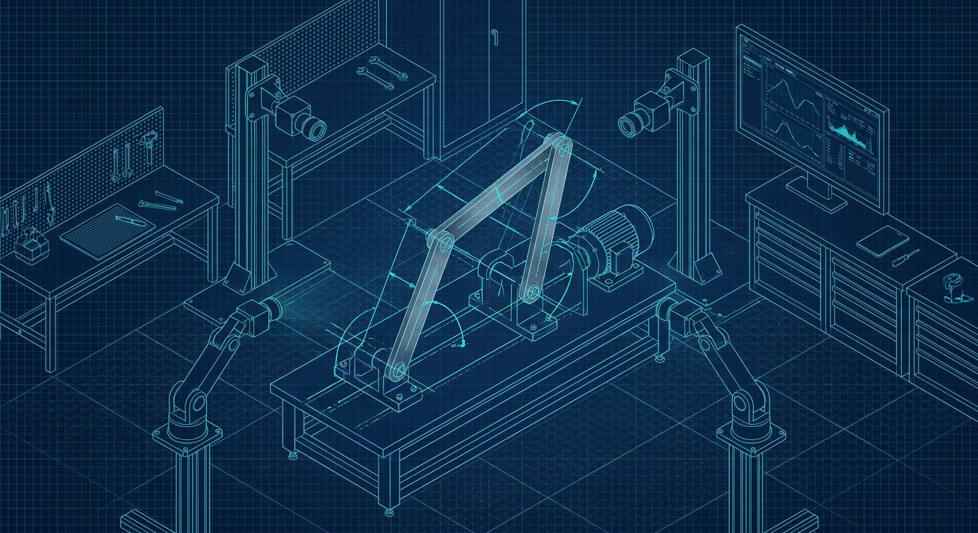
When a custom mechanical feed linkage built in 1984 finally shears a pivot pin on an automated packaging line, the maintenance log usually reveals two bad options. Option one is shutting down the line for twenty-four hours, pulling the entire assembly apart with bearing pullers, and hauling greasy links to a coordinate measuring machine (CMM) room. Option two is bringing in a handheld 3D laser scanner, capturing a dense, million-polygon surface mesh of the assembled mechanism, and discovering that the scan tells you nothing about where the internal shaft centerlines actually sit under load.
Neither path solves the real engineering problem. Plant managers do not want raw polygon meshes or forty hours of line downtime. They need the true kinematic chain: link lengths, revolute joint axes, degrees of freedom, stroke limits, and joint wear.
Recent work from Columbia University's Creative Machines Lab points toward a third route. Researchers led by Hod Lipson and Yuhang Hu published a framework where a robotic arm constructs its own internal kinematic model purely from multi-view video. The system observes its own motion across multiple camera angles, detects joint hierarchies, and calculates forward kinematics without CAD drawings or human kinematic trees.
For machine designers and shop-floor problem solvers, the implications reach far beyond autonomous robotics. The mathematics used to let an arm understand its own limbs provides a non-invasive blueprint for reverse-engineering undocumented, high-cycle factory machinery while the equipment stays bolted to the concrete.
The High Cost of Dead Geometry
Most modern reverse engineering workflows are built for static parts, not dynamic mechanisms. When an engineering team needs to duplicate or redesign a legacy mechanism, standard optical or structured-light scanners create a massive point cloud of the outer shell.
That shell is geometrically dense but kinematically dead.
A surface scan captures the outside of a cast-iron pillow block, the grime on an oil seal, and the visible head of a shoulder bolt. It does not identify the true center of rotation hidden inside the bearing bore. If the mechanism is a multi-bar linkage with four, six, or eight interconnected links, a static scan leaves the designer guessing at center-to-center distances.
If you miscalculate a pivot center-to-center dimension on a 4-bar planar linkage by just 0.4 mm, the rocker output error can amplify dramatically across its stroke. A mechanism designed to reach top dead center at 180 degrees of crank rotation might bind at 178 degrees, stalling an electric motor or overloading a gearbox.
Physical teardown avoids this by measuring bare parts directly on granite surface plates with height gauges and CMM probes. But teardown carries stiff costs:
- Production line downtime running between $800 and $5,000 per hour depending on plant throughput.
- Press fits, tapered pins, and dowels often deform or gall during extraction, altering the very clearances you want to measure.
- Static parts measured at room temperature on a CMM do not reveal dynamic deflection, play, or mechanical backlash caused by years of bore ovalization.
Visual kinematic reconstruction bridges this gap. By observing the mechanism moving through its operating cycle under power, optical tracking extracts operational kinematics directly from motion paths.
How Optical Self-Modeling Solves Kinematic Topology
The Columbia research team faced a problem familiar to every plant engineer: how do you build a working mathematical model of a mechanism when you have zero prior geometry?
In the Columbia setup, an arm with unknown joint configurations performed a series of exploratory motions while recorded by five streaming cameras. A neural network processed the visual feeds to map out continuous 3D coordinate transformations. The software determined where joints existed, which links were connected in series, and how joint angles mapped to end-effector positions.
To apply this technique to factory linkages, you do not need deep neural networks guessing abstract concepts. You need the underlying geometry engine: multi-view feature tracking converted into constrained kinematic fits.
Every rigid link in a planar or spatial mechanism has surface points that trace specific geometric paths during operation:
- Pure rotation about a fixed revolute joint produces a true circular arc in space.
- Points on a coupler link (connecting two moving pivots) trace complex algebraic curves, such as trochoids or higher-order coupler curves.
- Points on a slider or linear guide produce straight line vectors.
When you record a mechanism with two or three calibrated high-speed cameras, you can track distinct surface features on each moving link. By calculating the 3D trajectories of at least three non-collinear points per rigid body, you reconstruct the full SE(3) transformation matrix (rotation and translation) for that link across every frame of video.
Once the transformation matrix of each link is known across the cycle, calculating joint axes is a deterministic mathematical problem.
[Video Capture: 2-3 Sync Cameras]
             │
             ▼
[3D Point Cloud Trajectory Extraction]
             │
             ▼
[Spatial Motion Matrix per Rigid Link: SE(3)]
             │
             ▼
[Least-Squares Cylinder/Circle Arc Fitting]
             │
             ▼
[Joint Axis Vectors & Centerlines]
             │
             ▼
[Kinematic Graph: Links, Pivots, Bounds]
             │
             ▼
[Parametric CAD Assembly with Mates]
Solving Pivot Centerlines from Motion Arcs
To find the rotational centerline connecting Link A and Link B, you calculate the relative motion matrix between them. In an ideal revolute joint, all points on Link B rotate around a single fixed axis relative to Link A.
In mathematical terms, the relative displacement between the two links for any time step can be expressed as a screw displacement. According to Mozzi and Chasles' theorem, any rigid body displacement is equivalent to a rotation around an axis followed by a translation along that same axis. For a pure revolute joint, the pitch of that screw is zero.
By taking twenty to fifty discrete position samples across a mechanism stroke, an engineer can fit a spatial cylinder to the point trajectories using non-linear least squares (such as the Levenberg-Marquardt algorithm). The central axis of that fitted cylinder represents the true operational centerline of the pivot pin.
This delivers several distinct advantages over a standard 3D scan:
- Insensitivity to external geometry: It does not matter if the link is a raw forging, a welded tube, or covered in grease. As long as rigid surface points are trackable, the calculated center of rotation is exact.
- Built-in averaging of runout: Optical tracking samples hundreds of frames per cycle, averaging out high-frequency vibrations and sensor noise to find the true mean rotation axis.
- Detection of non-parallel axes: If a machine is binding because two pivot pins were welded out of parallel by 1.2 degrees, cylinder fitting will immediately flag the angular misalignment between the two calculated vectors.
Extracting Dynamic Backlash and Joint Wear
One of the most powerful aspects of optical kinematic tracking is its ability to measure joint degradation without pulling pins.
In an ideal 4-bar linkage with zero clearance, the position of the driven link is a strict, single-valued function of the input crank angle. However, real factory linkages run on bronze sleeve bearings, needle rollers, or spherical rod ends. Over millions of cycles, bearing bores develop radial play (clearance) and oval wear.
When a mechanism changes direction or transitions from tension to compression, that joint clearance produces mechanical backlash. The driving link moves through a small angle while the driven link remains stationary until the internal pin contacts the opposite wall of the worn bushing.
By comparing the kinematic path of the mechanism during the forward stroke against the return stroke, an optical tracking system reveals a distinct hysteresis loop.
Driven Link Angle (deg)
        ▲
        │                 / (Forward Stroke)
        │                /
        │               /  ◄─── Backlash Gap (Δθ)
        │              /  /
        │             /  /
        │            /  /  (Return Stroke)
        │           /  /
        │          /  /
        └─────────┴──┴──────────────► Crank Angle (deg)
The width of this hysteresis band (Δθ), mapped back through the link geometry, gives the exact radial clearance inside the joint under operating load. If an engineer knows the nominal pin diameter is 25.0 mm and the optical hysteresis calculates a 0.35 mm radial displacement under load reversal, they know immediately that the bushing is worn past standard running fit tolerances (such as an H7/f7 fit, which typically demands less than 0.05 mm clearance on that size) without ever putting a micrometer on the part.
Implementation Comparison: CMM vs 3D Scan vs Optical Tracking
To evaluate how this pipeline functions in a practical maintenance or rebuild scenario, consider an illustrative composite based on a standard 4-bar packaging feed linkage operating at 120 cycles per minute.
| Evaluation Metric | Traditional Teardown & CMM | Handheld 3D Laser Scan | Multi-View Optical Kinematics |
|---|---|---|---|
| Line Stoppage Required | 12 to 24 hours | 1 to 2 hours | 15 to 30 minutes |
| Output Data Format | Discrete point inspection report | Non-parametric STL / OBJ mesh | Vector kinematics & link lengths |
| Pin Centerline Accuracy | +/- 0.005 mm (isolated parts) | +/- 0.250 mm (estimated from mesh) | +/- 0.040 mm (dynamic mean axis) |
| Direct Backlash Detection | No (requires dial indicators) | No (static capture only) | Yes (hysteresis cycle extraction) |
| CAD Usability | Manual sketch rebuild required | Mesh wrapping / surface reconstruction | Direct input for parametric mates |
| Risk of Assembly Damage | High (bearing pullers, press fits) | Zero | Zero |
Note: Metrics represent an illustrative composite comparing standard plant rebuild workflows on a 4-bar steel mechanism with 400 mm nominal link lengths.
While a CMM delivers unmatched precision on an individual, disassembled component, it isolates the part from system-level compliance, mounting flexure, and dynamic clearance. Visual kinematic extraction captures the reality of the machine as it actually runs.
The Step-by-Step Shop Pipeline: From Video to Parametric CAD
To execute optical kinematic reverse engineering on a shop floor without custom robotics research software, mechanical designers can follow a five-stage workflow using accessible tools.
Stage 1: Optical Rigging and Calibration
Mount at least two high-speed cameras (minimum 120 frames per second to eliminate motion blur on links moving at 1-2 m/s) on rigid tripods isolated from machine frame vibrations. Ensure camera angles intersect between 60 and 90 degrees relative to the mechanism plane.
Place an accurate physical scale bar with high-contrast optical targets inside the field of view to define real-world millimeter scale and world coordinate axes. Apply high-contrast dot stickers or optical crosshairs to each moving link, placing at least three non-collinear markers per rigid body.
Stage 2: Trajectory Capture and Triangulation
Record three to five continuous operational cycles. Using open-source tracking tools or computer vision libraries (such as OpenCV), extract the 2D pixel coordinates of each marker across all frames.
Apply standard stereo-triangulation algorithms using camera calibration parameters (distortion coefficients, focal length, extrinsic rotation/translation matrices) to convert 2D pixel tracks into continuous 3D coordinate paths $(X(t), Y(t), Z(t))$.
Stage 3: Rigid Body Segmentation and Arc Fitting
Group markers belonging to the same physical link. Because the distance between markers on the same rigid body must remain constant, use a distance-invariance check across all time steps to filter out tracking noise or marker occlusion.
For each pair of adjacent links, calculate the relative transformation matrix. Fit a spatial circle or cylinder to the relative trajectory data using a non-linear least-squares algorithm to extract:
- Joint axis unit vector: $\mathbf{\hat{u}} = [u_x, u_y, u_z]^T$
- Pivot center coordinates: $\mathbf{P_0} = [x_0, y_0, z_0]^T$
- True kinematic link length: the Euclidean distance between pivot centers $\mathbf{P_A}$ and $\mathbf{P_B}$.
Stage 4: Wear and Backlash Quantification
Plot input driver position against driven link position across both halves of the stroke cycle. Measure the phase shift and angular lag at motion inflection points. Convert angular play to linear bearing wear using the calculated link radii.
Stage 5: Parametric Assembly Generation
Instead of importing raw meshes into CAD and attempting to fit sketches against faceted surfaces, export the extracted kinematic parameters directly:
- Generate standard parametric sketches in CAD using the exact center-to-center link distances.
- Define standard cylindrical pin mates along the calculated joint axis vectors.
- Apply engineering fit tolerances (such as H7 bore tolerances and g6/h6 pin tolerances) informed by the measured backlash data.
- Run a motion simulation inside the CAD environment to verify that stroke limits, transmission angles, and dead points match the high-speed video recording.
Practical Failure Modes and Field Limitations
Optical kinematic reconstruction is a powerful tool, but treating it like magic leads to ruined tooling. Mechanical engineers must recognize several sharp constraints before relying on video-derived data.
Out-of-Plane Deflection and Structural Compliance
Machine linkages are not perfectly rigid. Under high acceleration or cutting loads, slender steel links experience elastic bending. If optical markers flex out of plane by 0.5 mm during peak acceleration, standard rigid-body arc fitting will interpret that elastic deflection as joint wear or an off-axis pivot.
To combat this, record calibration cycles at low machine speeds (jog mode) to establish baseline rigid kinematics, then record full-speed production cycles to measure dynamic structural compliance.
Optical Occlusion and Harsh Environments
Factory linkages rarely operate in clean, well-lit spaces. Coolant mist, guarding panels, hydraulic lines, and particulate matter frequently obscure tracking markers. If a marker disappears behind a safety plate for thirty percent of its stroke, the circle-fitting algorithm must extrapolate across the gap, which increases axis location error. Use high-intensity LED panel lights and polarized camera filters to cut through cutting fluid and oil sheen.
Lens Distortion and Calibration Drift
Standard wide-angle lenses introduce barrel distortion that warps trajectory lines toward the edges of the image sensor. If you fail to calibrate lenses using a precision checkerboard or dot grid target at the exact working distance of the mechanism, a straight slider track will register as a curved path in 3D space, corrupting the kinematic model.
What this means for Mexaio AI
Generative mechanical engineering cannot rely on uneditable, static surface meshes. The core insight from Columbia's self-modeling research is that mechanisms are defined by their functional motion, degrees of freedom, and constraint graphs, not just their outer skins.
Mexaio AI is built around this exact principle. When mechanical designers extract kinematic skeletons from legacy equipment or synthesize entirely new mechanisms from scratch, the platform does not produce dead polygon geometry. It produces parametric, fully editable CAD assemblies equipped with valid mate relationships, precise center-to-center linkages, and verified motion envelopes.
By uniting kinematic synthesis with realistic dynamic simulation, Mexaio AI ensures that when an engineer designs or reconstructs a linkage, every joint clearance, transmission angle, and machine fit is ready for direct manufacturing on CNC mills and wire EDM machines.
Moving from Theory to the Shop Floor
Reverse engineering legacy plant mechanisms does not require choosing between catastrophic production downtime and useless static surface scans. The math developed to give autonomous robots self-awareness provides mechanism designers with a non-destructive, highly precise method for extracting kinematic truths from moving machinery.
Before you take a torch or a puller to your next undocumented packaging machine or transfer press, mount two high-speed cameras, affix tracking dots to the link pivots, and record ten seconds of clean motion. Extract the rotation arcs, calculate the true centerlines, and build parametric CAD models driven by real physics rather than guesswork.
Sources
- Columbia Engineering: Robots Learn How to Move By Watching Themselves
https://www.engineering.columbia.edu/about/news/robots-learn-how-move-watching-themselves-0 - Creative Machines Lab (Columbia University): Visual Self Modeling
https://www.creativemachineslab.com/visual-self-modeling.html - Tech Briefs: How Do Robots Learn? By Watching Themselves
https://www.techbriefs.com/component/content/article/53373-how-do-robots-learn-by-watching-themselves - Science Robotics / Tech Xplore: Engineers build a robot that learns to understand itself
https://techxplore.com/news/2022-07-robot-world.html - ScienceDirect Topics: Kinematic Chains and Linkage Analysis
https://www.sciencedirect.com/topics/engineering/kinematic-chain