Why AI Autorouters Pass DRC but Fail High Speed Signal Integrity

AI layout engines hit 100 percent DRC completion with ease, but geometric clearance does not guarantee signal integrity. Here is how to catch high-speed bus failures before fab.

Recent public layout evaluations and community benchmarks, including test suites like EEBench and discussions across engineering forums, show modern generative PCB engines and reinforcement learning routers routinely achieving 100 percent net completion. They route dense mixed-signal boards in minutes and return zero errors on native Design Rule Checking (DRC). To an engineering manager reading an automated sign-off report, the layout looks ready for the fabrication panel.

Then the prototype arrives from assembly. The microcontroller boots, power rails settle at nominal voltages, and low-speed UART works. But the moment the firmware brings up a USB 3.2 Gen 1 link, an RGMII Ethernet bus, or a 50-ohm RF trace, the link drops packets, exhibits severe eye-diagram closure, or fails radiated emissions compliance entirely.

For a solo hardware lead or an early-stage hardware startup, this failure is catastrophic. A four-to-six-layer impedance-controlled turn with quick-turn SMT assembly costs anywhere between $2,500 and $6,000 per iteration. Losing two to three weeks waiting for replacement boards burns precious runway. More dangerously, diagnosing an intermittent high-speed failure on physical hardware consumes weeks of bench time with high-bandwidth oscilloscopes and time-domain reflectometers.

Passing DRC simply means a trace does not violate 2D and 3D manufacturing clearance limits. It does not mean the trace behaves as a functional transmission line. Understanding why machine learning routing architectures generate this blind spot is the first step toward catching electrical failure modes before sending Gerber or ODB++ files to the fab.

The Fundamental Disconnect Between Geometry and Maxwell's Equations

Traditional and AI-driven autorouters treat PCB layout primarily as a topological pathfinding problem. Reinforcement learning (RL) models and geometric graph search algorithms are optimized around discrete reward functions: minimize total trace length, minimize via count, eliminate clearance violations, and achieve 100 percent completion.

Modern EDA clearance checkers verify static geometric constraints. They calculate point-to-point euclidean distances between copper features on the same layer, check drill-to-copper spacing, confirm solder mask expansion, and ensure trace widths match the netclass rule. If a differential trace is defined as 0.127 mm wide with a 0.127 mm gap, and it stays at least 0.150 mm away from adjacent digital lines, the DRC engine issues a green checkmark.

Electrons traveling at high frequencies do not operate on netlist topology alone. At frequencies where signal rise times are shorter than twice the electrical propagation delay across the trace (typically anything above 50 to 100 MHz on standard FR-4), the return current flows through the path of least inductance, not the path of least resistance. That return current gathers directly underneath the signal conductor on the nearest continuous reference plane.

When an AI router navigates congested component pin-outs, it moves traces across layers to evade obstacles. To the routing model, a copper plane on Layer 2 and a copper plane on Layer 5 are interchangeable geometric escape paths. The router drops a signal via, swaps layers, and continues running the trace. If no other net violates copper-to-copper spacing, the geometric check passes.

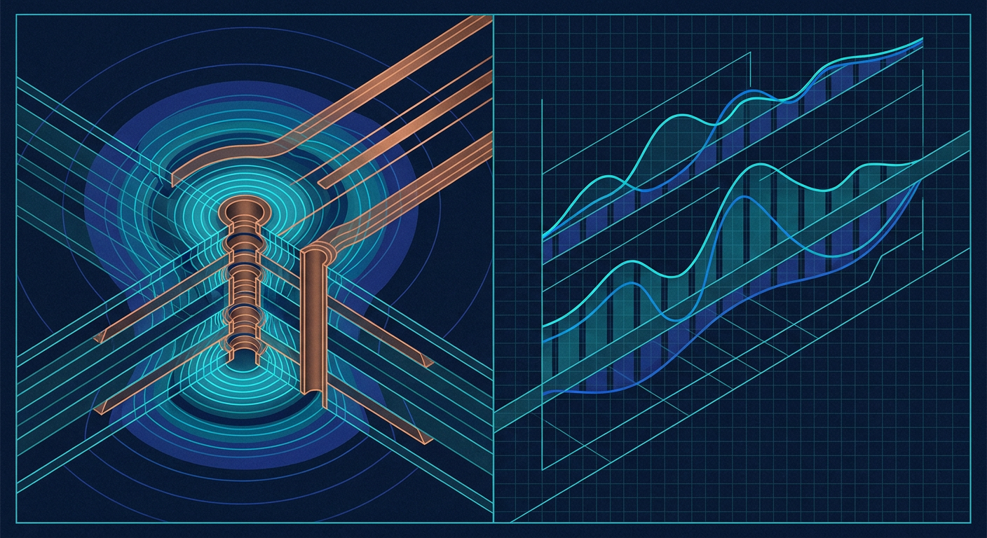
Electromagnetically, that via switch just forced the high-frequency return current to find an alternate path back to its reference plane. If the router did not place an adjacent ground stitching via within a fraction of a wavelength, the return current detours across power planes, through distant decoupling capacitors, or across anti-pad voids. The result is an inductive loop that destroys controlled impedance, causes high-frequency ringing, injects crosstalk into neighboring circuits, and radiates electromagnetic interference.

Three Silent High-Speed Failure Modes in Clean DRC Layouts

When inspecting machine-generated layouts that achieved clean DRC status, signal degradation typically concentrates in three specific physical layout features: reference plane slotting, uncompensated via transitions, and copper balance starvation.

1. Anti-Pad Merging and Reference Plane Rupture

Dense BGA breakouts and pin headers require dozens of vias clustered tightly together. Standard fabrication design rules specify minimum drill-to-copper clearance for internal power and ground planes to prevent short circuits during drilling tolerances. This clearance creates a circular void in the copper plane around the via barrel, known as an anti-pad.

When an AI autorouter routes a bus through a tight pin matrix, it places multiple vias in close proximity. While each individual via complies with fab clearance rules, the overlapping anti-pads merge into a continuous copper cutout inside the ground plane.

The autorouter sees Layer 2 as a valid reference plane because the plane polygon exists in the CAD database. However, the signal trace on Layer 1 is now flying over a physical slot in the ground return plane. The characteristic impedance jumps instantly from 50 ohms to over 90 ohms. The return current cannot cross the void; it diverts around the perimeter of the cutout, forming a large loop antenna. A standard DRC engine will never flag this because it evaluates the copper clearance of each via independently against the polygon, without calculating the topological continuity of the return path beneath the trace.

2. Uncompensated Layer Transitions and Via Stubs

Changing routing layers is the easiest way for an automated pathfinding algorithm to resolve track collisions. Human layout specialists avoid layer transitions on critical high-speed nets, preferring to keep critical lines on a single microstrip or stripline layer with an unbroken ground plane. When a transition is unavoidable, a human engineer manually places a ground stitching via directly beside the signal via to preserve the return path geometry.

Generative and RL routers often drop two, four, or six vias along a single high-speed trace to navigate dense routing channels. In a typical 6-layer stackup (Top-GND-Sig1-Sig2-PWR-Bottom), transitioning a trace from Top to Sig1 changes the reference plane from Layer 2 to Layer 2/Layer 5. If the trace transitions from Top to Bottom, the return current must transfer from the Layer 2 ground plane to the Layer 5 power plane.

Without a nearby bypass capacitor or stitching via connecting the reference systems, this layer transition creates a major impedance discontinuity. Furthermore, on through-hole drilled boards, routing on internal layers leaves an unused barrel segment, known as a via stub. At multi-gigabit speeds, this stub acts as an open-ended transmission line that reflects energy back into the main trace at its resonant quarter-wavelength frequency, creating a deep notch in the channel insertion loss. The DRC tool sees only a compliant plated hole; it has no concept of resonance or stub-induced signal attenuation.

3. Asymmetric Copper Starvation and Differential Skew

Differential signaling relies on matched electrical lengths, consistent common-mode rejection, and symmetrical electromagnetic coupling between positive and negative traces. While automated engines excel at matching total geometric trace lengths through serpentine tuning patterns, they frequently break the physical symmetry of the differential environment.

An RL router attempting to escape a dense microcontroller pinout will often separate differential pairs around intermediate vias, or run one leg of the pair over a solid ground fill while routing the other leg over a split power boundary. Both traces report identical physical lengths to the millimeter in CAD constraint managers, satisfying length-matching rules.

However, because the phase velocity of an electromagnetic wave depends on the effective dielectric constant of its surrounding medium, the leg running over the discontinuous copper experiences a lower effective capacitance and a different propagation delay. The physical lengths match, but the electrical delay skews. This intra-pair skew converts differential signals into common-mode noise, degrading receiver eye height and increasing radiated emissions.

Receipts: Automated Routing vs Signal Integrity Metrics

To understand the performance gap between raw geometric compliance and high-speed electrical validity, consider an illustrative composite benchmark representing typical results observed when routing high-speed digital buses (PCIe Gen 3 at 8 Gbps, DDR4 at 2400 MT/s, and USB 3.2 Gen 1 at 5 Gbps) across standard 6-layer FR-4 stackups using baseline geometric RL autorouting versus physics-aware placement and routing.

Evaluation Metric	Geometric RL Autorouter	Physics-Aware Layout Sign-Off	Target Specification
Native 2D/3D DRC Errors	0 Violations	0 Violations	0 Violations
Net Completion Rate	100%	100%	100%
Unstitched Layer Transitions	14 per bus (average)	0 per bus (strictly paired)	0 unstitched transitions
Differential Impedance Spikes	82 Ω to 118 Ω (±28%)	94 Ω to 104 Ω (±4%)	100 Ω ± 10% tolerance
Return Path Discontinuities	6 plane crossings	0 plane crossings	0 crossings over split planes
Eye Height Margin (PCIe Gen 3)	42 mV (Fails Mask)	168 mV (Passes Mask)	≥ 120 mV at 10⁻¹² BER
Estimated Respin Probability	70% to 90%	< 5%	0% first-pass failure

Note: This data is an illustrative composite based on high-speed channel simulations run across standardized 6-layer test stackups (1.6mm FR-4, 0.5 oz outer, 1 oz inner copper) comparing pure geometric clearance outputs against 3D quasi-static electromagnetic verification standards.

The data illustrates the primary trap: both pipelines deliver a 100 percent complete, zero-DRC board. But the pure geometric layout produces transmission line discontinuities that close the receiver eye diagram, ensuring that the manufactured board will fail functional validation on the test bench.

Practical Verification: Auditing AI Layouts Before CAM Dispatch

If you use AI routing engines to accelerate your layout workflow, treat candidate layouts as rough drafts rather than manufacturing-ready files. Before generating Gerbers or authorizing an expensive assembly run, solo engineers should execute a strict, manual verification protocol focused on electromagnetic return paths.

Step 1: The Negative-Space Plane Audit

Turn off all signal layers in your CAD viewer and inspect only your internal ground reference layers (typically Layer 2 and Layer 5 in a standard 6-layer stackup). Look for regions where via clusters create perforated rows or merged slots. If a continuous high-speed signal trace on an adjacent outer layer crosses one of these cleared zones, the layout must be corrected. Either spread the via pitch to maintain copper webs between anti-pads or manually reroute the high-speed traces around the perforation.

Step 2: Via Transition Stitching and Ground Transfer Verification

Isolate your high-speed nets (USB, PCIe, Ethernet, MIPI, high-speed SPI, and clocks). Trace each net from driver to receiver and count the via transitions. Every time a high-speed net drops through a via to an alternate reference layer, verify the presence of a ground stitching via placed within 0.5 mm to 1.0 mm of the signal via. If the transition changes reference planes across different DC potentials (for instance, from a ground-referenced microstrip to a power-referenced stripline), ensure a low-ESR ceramic decoupling capacitor (0.1 µF in 0402 or 0201 package) is placed directly adjacent to the transition to provide a high-frequency AC return path.

Step 3: Split Plane Boundary Check

Overlay all power plane split boundaries against your critical signal layers. AI autorouters regularly drag traces across 3.3V, 1.8V, and 1.2V island boundaries on internal power layers. Ensure that no trace carrying edge rates faster than 1 ns crosses any split plane boundary. If a signal must travel across multiple voltage domains, keep it strictly referenced to an unbroken ground plane on an adjacent continuous layer.

Step 4: Stacking and Copper Balance Inspection

Automated routing engines often cluster traces tightly on one side of a board while leaving large empty areas on the other. This creates significant copper imbalance across the panel. During fabrication, unbalanced copper distribution causes uneven thermal expansion during lamination and reflow, leading to board warpage, tombstoning of small passive components, and uneven etching that skews controlled impedance trace widths. Check your layer-by-layer copper density percentages and use hatch or solid copper thieving pours to balance non-signal areas.

Step 5: Live Sourcing and Component Package Validation

Verify that the pinout models used by the AI engine match the exact physical components in your live bill of materials (BOM). Generative systems frequently route traces assuming idealized pad dimensions or generic pin assignments. If your BOM calls for an ultra-compact QFN with an exposed thermal pad, ensure the router has not dropped unconnected signal vias through the ground pad without proper solder mask tenting or capping, which would cause solder wicking and assembly voids during SMT reflow.

How This Reshapes Autonomous PCB Design

The engineering challenge of the next five years is not teaching computers how to draw lines between coordinates without touching. That is a solved geometric optimization problem. The real challenge is integrating full field electromagnetic physics, thermal behavior, and manufacturing assembly constraints directly into the layout synthesis loop.

When layout tools evaluate Maxwell's equations and return currents during the pathfinding phase, rather than running a superficial clearance check at the end, autorouting shifts from an experimental toy into a reliable production tool. This is the design philosophy driving IntelCAD, where automated layout generation is coupled directly to physics-aware constraints, live supply chain availability from global distributors, and real-world DFM validation.

Treating DRC as the finish line is the most expensive mistake a hardware team can make. Until autorouting systems natively simulate electromagnetic return currents and high-speed transmission dynamics, the human engineer's primary job is verifying the physics that geometric rules ignore.

Why do AI autorouters pass DRC checks while failing on high-speed signals?

Traditional DRC only evaluates 2D and 3D manufacturing tolerances, such as minimum trace spacing, annular ring widths, and drill clearances. It does not evaluate transmission line physics, electromagnetic field boundaries, return current paths, or via stub resonances. AI autorouters optimize for geometric clearance and completion, which allows them to achieve zero DRC errors while inadvertently creating severe return path ruptures, impedance spikes, and differential skew.