ABB Robotics recently launched RobotStudio HyperReality, integrating NVIDIA Omniverse libraries into its simulation pipeline to claim up to 99 percent sim-to-real accuracy and an 80 percent reduction in commissioning time. For robotics integrators and machine builders, the promise is seductive: validate cycle times, motor thermal envelopes, and path precision in a virtual world before ordering custom actuators or machining mechanical arms.
Yet mechanism designers running high-speed parallel linkages, crank-sliders, and custom pick-and-place kinematics know where the virtual twin falls apart. A standard rigid-body physics engine can calculate gross inertia, coordinate transforms, and idealized contact points with remarkable speed. But when a four-bar linkage accelerates at 20G to hit a 120-cycle-per-minute target, nominal joint models miss the real mechanical world entirely.
Pin friction under dynamic load, micro-slip in press-fit needle bearings, link flexure under peak reversal torque, and thermal growth inside bushing housings do not obey idealized Coulomb friction sliders. If your design office trusts default simulation numbers without physical damping calibration, your real machine will miss position targets, overheat its servo drives, or shake its mounting plate to pieces within forty-eight hours of shop-floor commissioning.
Where Rigid-Body Solvers Drop the Mechanical Physics
Most commercial robotics simulation platforms, including offline programming suites driven by gaming or graphics physics engines, resolve multi-body systems using iterative linear complementarity problem (LCP) solvers or maximal-coordinate Featherstone algorithms. These numerical engines assume links are infinitely stiff, pin joints rotate around mathematically perfect central axes, and friction is a single constant coefficient multiplied by normal force.
On a machine shop floor, an acceleration cycle turns those assumptions upside down.
Consider an aluminum 7075-T6 rocker arm driven by an AC brushless servomotor through a planetary gearbox. When the servo commands a trapezoidal velocity move with a 15-millisecond acceleration ramp, the peak torque applied to the input crank can exceed the steady-state running torque by 400 to 600 percent.
Under that violent surge, three distinct physical phenomena occur simultaneously in the joint:
- Dynamic load shift on joint pins. The normal force vector inside the needle roller or bronze sleeve bearing swings through 180 degrees in a fraction of a second. This forces the lubricating grease or oil film into boundary friction regime, causing instantaneous friction torque spikes that standard constant-friction models ignore.
- Bushing and housing elastohydrodynamic collapse. Under instantaneous contact pressures exceeding 40 MPa, the lubricant film thins out. The joint transitions along the Stribeck curve from hydrodynamic lubrication into mixed or boundary friction, dramatically increasing resistive torque right at the moment of peak servo demand.
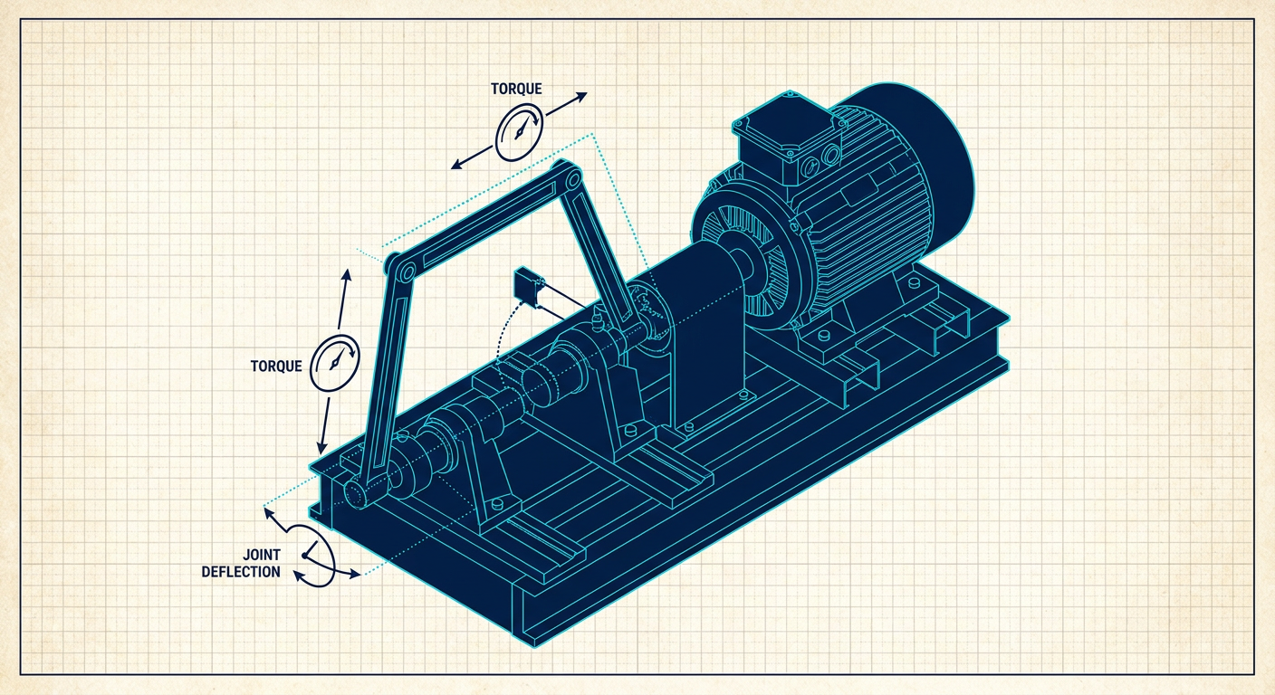
- Link compliance and phase lag. The physical link flexes elastically. As the link bends by even 0.15 mm under peak inertial loading, the effective kinematic center of the pin rotates out of alignment with its mating clevis. This angular misalignment causes edge-loading on the bearing track, doubling local friction and creating stick-slip vibrations as the arm tries to settle at the target coordinate.
When these effects combine, the actual motor torque required to complete the trajectory does not match the simulation trace. The servo drive hits current limits, tracking error faults trip the controller, and the robot fails to achieve its simulated cycle time.
The Mathematical Friction Gap in Fast Kinematic Chains
To see why standard simulations drift from bench reality, examine how joint friction torque is calculated in software versus what a physical dynamometer registers.
The Classical Simulation Equation
Most multi-body simulation tools model revolute joint friction torque $T_f$ with a simplified Coulomb plus viscous damping formulation:
$$T_f = \mu \cdot F_N \cdot r_{pin} + c_v \cdot \dot{\theta}$$
Where:
- $\mu$ is a constant friction coefficient (often set between 0.02 and 0.08 for rolling bearings).
- $F_N$ is the scalar magnitude of the calculated joint reaction force.
- $r_{pin}$ is the pin radius.
- $c_v$ is a constant viscous damping coefficient.
- $\dot{\theta}$ is the joint angular velocity.
This equation is smooth, computationally cheap, and entirely stable in real-time solvers. It is also physically incomplete for high-acceleration linkages.
The Real-World Dynamic Joint Behavior
On physical hardware, joint resistive torque is a non-linear function of load direction, velocity, lubricant viscosity, thermal state, and structural clearance:
$$T_f(t) = \left( T_c + (T_s - T_c) e^{-|\dot{\theta} / \dot{\theta}s|^{\delta}} \right) \operatorname{sgn}(\dot{\theta}) + c_v \dot{\theta} + T{edge}(\alpha_{def}) + T_{stack}(\Delta_{fit})$$
Where:
- $T_s$ is the static breakaway friction torque under dynamic clamping load.
- $T_c$ is the Coulomb friction torque.
- $\dot{\theta}_s$ is the Stribeck velocity threshold.
- $\delta$ is the Stribeck exponent (typically between 1.0 and 2.0).
- $T_{edge}(\alpha_{def})$ is the additional friction torque induced by angular deflection $\alpha_{def}$ of the pin inside the clevis under bending load.
- $T_{stack}(\Delta_{fit})$ is the internal preloading torque caused by machining tolerance stack-up and thermal expansion of the housing bore.
When an arm reverses direction at top dead center, $\dot{\theta}$ crosses zero. At that exact transition, the Stribeck exponential term produces an abrupt resistance spike while the joint breaks out of static friction. If the simulation engine uses a simple velocity-damping curve to prevent numerical jitter, it smooths away this breakaway spike. The simulation shows a clean, effortless reversal; the actual machine sees an impulse spike that rings through the drive train.
Measured Dynamics: Simulation Against the Bench
To demonstrate how wide this gap can be, the following illustrative composite compares simulated parameters against physical dynamometer measurements on a representative high-speed aluminum four-bar pick-and-place linkage driven at 120 cycles per minute.
Illustrative Performance Comparison: 4-Bar High-Speed Kinematic Cell
| Operational Metric | Standard Rigid-Body Sim | Calibrated Non-Linear Sim | Physical Bench Test (Dyno) | Deviation (Standard vs Physical) |
|---|---|---|---|---|
| Peak Input Torque (Acceleration) | 14.2 N·m | 21.8 N·m | 22.6 N·m | -37.2% |
| Peak Input Torque (Reversal) | 11.8 N·m | 18.4 N·m | 19.1 N·m | -38.2% |
| Settling Time at Endpoint (±0.05 mm) | 18 ms | 46 ms | 52 ms | -65.4% |
| Steady-State RMS Motor Current | 4.8 A | 6.7 A | 7.1 A | -32.4% |
| Joint Operating Temperature Rise (30 min) | N/A (Assumed 20°C) | +22°C modeled | +26°C measured | Complete omission |
| End-Effector Overshoot at 1.5 m/s | 0.08 mm | 0.34 mm | 0.38 mm | -78.9% |
Note: This data represents an illustrative composite based on standard industrial servo-driven four-bar testbench architectures using 7075-T6 aluminum arms, preloaded deep-groove ball bearings, and planetary drive reduction (10:1 ratio).
Notice the pattern. The standard rigid-body simulation underestimated the peak torque required during acceleration by more than 37 percent. Why? Because it assumed the bearings remained in pure rolling contact at low nominal friction, ignored the momentary compliance in the driven arm, and treated the pin joints as frictionless constraint pivots.
When the design team purchases a motor sized for 15 N·m peak capability based on the standard simulation, the real hardware triggers an overcurrent alarm on its very first production-rate run.
Calibrating Virtual Physics Before Machining Parts
If you want your mechanism simulation to match the real machine shop result, you cannot rely on default physics engine presets. You need a systematic calibration workflow that extracts real joint damping and compliance parameters before cutting metal or freezing actuator selections.
1. Characterize Dynamic Bearing Friction Under Lateral Thrust
Do not rely on the catalog static friction rating $C_0$ or basic dynamic load rating $C$ to guess joint drag. Bench-test the actual bearing assembly (whether it is an INA needle roller, an Igus composite sleeve, or an SKF deep-groove pair) under static lateral loads equivalent to your mechanism peak inertial forces.
Mount the pin and bearing block in a hydraulic press or rigid test jig, apply the calculated peak radial force with a calibrated load cell, and measure the torque required to oscillate the pin through your operating angle using a torque wrench or reaction torque sensor. Feed that empirical friction-versus-load slope back into your joint property cards.
2. Measure Joint Damping via Ring-Down Step Testing
To capture structural and joint damping accurately:
- Assemble a single link with its actual pivot bearings and clamping bolts torqued to specification.
- Lock the base firmly to a heavy cast-iron surface plate.
- Deflect the free end of the link by a known displacement within its elastic limit and release it cleanly.
- Record the oscillation decay using an accelerometer or a non-contact laser displacement sensor.
Calculate the logarithmic decrement $\delta_{decay}$ from successive peak amplitudes $x_n$ and $x_{n+1}$:
$$\delta_{decay} = \ln\left(\frac{x_n}{x_{n+1}}\right)$$
$$\zeta = \frac{\delta_{decay}}{\sqrt{4\pi^2 + \delta_{decay}^2}}$$
This dimensionless damping ratio $\zeta$ captures both material hysteresis and joint interface dissipation. Insert this measured damping factor directly into your simulation dynamics solver rather than leaving viscous damping at zero.
3. Account for Housing Bore Fit Tolerances
Machining tolerances have a massive impact on pin friction. An ISO H7 bore in an aluminum link housing paired with an h6 ground pin gives a clearance fit of +0.000 to +0.025 mm at room temperature.
However, when the mechanism runs continuously, thermal expansion in the aluminum housing (coefficient of thermal expansion $\approx 23 \times 10^{-6} / \text{K}$) expands the bore faster than a steel pin ($\approx 12 \times 10^{-6} / \text{K}$). Conversely, if you are pressing a thin-walled steel bushing into an aluminum clevis with an interference fit (e.g., ISO N6/h6), housing contraction at cold startup can squeeze the bushing internal diameter by 0.012 mm, pinching the pin and multiplying static breakaway torque by five.
Your kinematic model must evaluate both tolerance limits:
- Maximum Material Condition (MMC): Tighter fit, maximum pin diameter, minimum bore. This evaluates worst-case joint friction, motor thermal loading, and stick-slip stall risk.
- Least Material Condition (LMC): Loosest fit, maximum backlash, minimum pin diameter. This evaluates worst-case kinematic play, vibration settle times, and end-effector positioning error.
Designing Linkages for High Dynamic Fidelity
When designing fast mechanisms, adjusting software numbers is only half the battle. You should also design the physical geometry to minimize non-linear friction and compliance errors that simulators struggle to predict.
+-------------------------------------------------------------------------+
|                   HIGH-SPEED LINKAGE DESIGN RULES                       |
+-------------------------------------------------------------------------+
|  1. STRADDLE CLEVIS MOUNTING                                            |
|     Avoid cantilevered pins. Symmetric double-shear clevis mounts       |
|     eliminate pin bending and edge-loading on bearings.                 |
|                                                                         |
|  2. PRELOADED ANGULAR CONTACT PAIRS OVER SINGLE DEEP-GROOVE             |
|     Dual angular contact bearings with ground shims eliminate axial     |
|     micro-play and maintain predictable rotational friction under load. |
|                                                                         |
|  3. SECTION MODULUS OVER SOLID MASS                                     |
|     Use hollow structural profiles (e.g., 6061-T6 thin-wall box or      |
|     carbon fiber tube with bonded 7075 inserts) to maximize dynamic     |
|     stiffness without adding rotational inertia.                        |
|                                                                         |
|  4. BALANCED THERMAL INSERTS                                            |
|     When press-fitting steel bearings into light alloy links, use       |
|     symmetrical wall thicknesses around the bore to prevent out-of-     |
|     round distortion during thermal cycling.                            |
+-------------------------------------------------------------------------+
Cantilevered pin joints are the single biggest cause of unmodeled friction spikes in parallel robotics. When a cantilevered pin takes high lateral acceleration force, it acts as a short beam under moment load. The pin tilts by fractions of a millidegree inside the bearing bore, driving the contact stress toward the outer edge of the rollers.
A rigid-body physics simulator assumes the load remains uniformly distributed along the entire roller length. In the real machine, that edge concentration breaks the oil film, scuffs the raceway, and generates an unmodeled braking torque that degrades positioning accuracy.
By replacing cantilevered joints with double-shear straddle clevises, you force the pin to deflect in pure parallel bending, maintaining uniform bearing contact across the entire dynamic stroke.
What This Means for Mexaio AI
Tools like ABB RobotStudio HyperReality are pushing industrial simulation toward photorealistic and physically rich environments. But for engineers designing the actual mechanism hardware, photorealism is useless if the underlying geometry cannot be parametrically adjusted to solve dynamic mechanical failures.
Generative mechanical engineering cannot simply output static, dead boundary representation (B-rep) solids or polygon meshes that look like industrial arms. It must generate fully parametric, editable kinematic assemblies where joint constraints, clearance fits, bearing bore tolerances, and dynamic compliance are mathematically linked.
Platforms like Mexaio AI approach mechanism design from this engineering-first principle: generating kinematic geometry that is explicitly parameterized for real-world manufacturing constraints, fit classes, and dynamic loads. When a physical test or higher-order dynamic simulation reveals that a joint is deflecting or pinching under acceleration, the designer must be able to adjust wall thicknesses, clevis spans, and pin diameters parametrically in the CAD model without rebuilding the kinematic tree from scratch.
A Practical Checklist for Fast Mechanism Builds
Before you send linkage drawings to the CNC milling center or finalize servo motor frame sizes based on a virtual simulation, run through this verification checklist:
- Verify your friction safety factor. Take the peak torque calculated by your multi-body simulation and apply a minimum 1.4x factor to cover dynamic boundary lubrication spikes, bearing preloading, and seal drag during high-G reversals.
- Run both MMC and LMC tolerance stack simulations. Ensure that your motor can overcome the friction torque of the tightest allowable bearing press fit, while confirming that your settling time meets specification at the loosest allowable pin clearance.
- Calculate pin slope under peak inertial load. Check that maximum elastic bending of your pivot pin does not exceed the manufacturer allowable angular misalignment for your chosen bearing (typically less than 2 to 4 arcminutes for standard needle rollers).
- Extract empirical damping from physical coupons. If you are using carbon fiber composite links or 3D-printed titanium structures with bonded inserts, run a basic physical tap or ring-down test to extract real modal damping coefficients instead of relying on default software constants.
- Check dynamic seal drag. Lip seals on rotary joints can contribute up to 30 percent of total joint friction at low speeds. Measure seal breakout torque separately and include it as an explicit offset in your simulation model.
Sim-to-real tools are closing the gap on optical sensor simulation, ray-traced computer vision, and gross trajectory planning. But on the machine shop floor, physics still rules the pin joints. Measure your damping, calibrate your contact friction under realistic peak loads, and design your linkages with the stiffness required to make the real machine run as cleanly as the simulation on your screen.
Sources
[1] https://www.abb.com/global/en/news/134178/wbstr-closing-the-sim-to-real-gap-how-abbs-robotstudior-hyperreality-enables-industrial-scale-physical-ai [2] https://www.abb.com/global/en/areas/robotics/innovation/robotstudio-hyperreality [3] https://www.abb.com/global/en/areas/robotics/products/software/robotstudio-suite [4] https://claru.ai/blog/sim-to-real-gap [5] https://news.mit.edu/2026/ai-agents-create-virtual-playgrounds-to-help-robots-get-crucial-training-data-0713