At the IEEE International Conference on Robotics and Automation (ICRA), NVIDIA Research presented a series of papers addressing the persistent barrier in physical robotics: the sim-to-real gap in robotic manipulation and loco-manipulation. The headline demos from physics engines look clean. An artificial intelligence policy trained across millions of parallel simulated hours in Isaac Sim executes dynamic pick-and-place routines, high-speed catching, and complex tool orientation without dropping a frame.
Then that exact policy gets flashed onto a physical six-axis arm or a four-degree-of-freedom manipulator on the factory floor, and the hardware stalls mid-trajectory. The end effector overshoots by three millimeters, the wrist oscillates during rapid deceleration, and joint actuators pull twice their simulated current draw until thermal protection trips the drive controllers.
For mechanism designers, automation engineers, and robotics hardware startups, this disconnect is not a software surprise. It is a predictable failure of idealized mechanical assumptions. Physics engines overwhelmingly treat robot links as perfectly rigid bodies connected by frictionless mathematical hinges with simplified viscous damping terms. Real robotic joints run on strain wave gearing, planetary reducers, cross-roller bearings, and grease formulations whose shear dynamics change under load and temperature.
If you design arm linkages, size joint actuators, or prepare kinematics for automated motion planning, relying on default physics models will blow up your prototype budget. Bridging this gap requires treating joint compliance, harmonic drive friction spikes, and dynamic link deflection as first-class mechanical design constraints rather than downstream control problems.
The Real Mechanics Inside the Simulated Joint
Most robotic simulation pipelines define an arm using a Unified Robot Description Format (URDF) file. In a standard URDF, a revolute joint has an axis of rotation, upper and lower angular limits, a maximum velocity, an effort ceiling, and two scalar parameters: damping and friction.
When a reinforcement learning model trains against that joint, the simulator calculates torque as a simple linear function of angular velocity plus a constant Coulomb friction offset. In reality, strain wave gears (commonly referred to by the trade name Harmonic Drive) behave nothing like a linear damper.
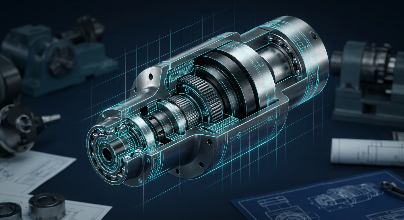
A strain wave gear relies on an elliptical wave generator rotating inside a flexible, externally toothed cup (the flexspline), which engages with an internal ring gear (the circular spline). Power transmission depends entirely on the continuous elastic deformation of alloy steel. That elastic interface introduces three physical phenomena that idealized simulators routinely ignore:
Load-dependent friction spikes. Friction inside a harmonic drive is not a fixed constant. As external payload torque increases, the radial force pressing the flexspline teeth into the circular spline rises dramatically. Under high cantilevered loads, normal contact forces multiply, causing friction torque to surge non-linearly. Simulators that assume constant friction drastically underestimate the torque required to break static friction during high-payload moves.
Stiction and the Stribeck effect at velocity reversals. When an arm decelerates to zero velocity to change direction, it transitions from hydrodynamic fluid lubrication in the gear teeth back into boundary and mixed lubrication. Breakaway torque can be three to four times higher than the running viscous friction. If the controller executes a fine positioning move near zero velocity, the joint sticks until motor winding current spikes, causing a sudden jerk forward that destroys precision.
Multi-stage torsional compliance. A harmonic drive is not rigid. Its torque-versus-torsion curve features three distinct stiffness zones. At low torque, the joint behaves like a soft spring with high hysteresis. As torque rises through the intermediate range, the flexspline teeth fully seat and stiffness climbs. Under peak acceleration or shock loads, the system enters a high-torque spring zone.
Ideal Simulated Joint:     [Motor] === (Rigid Axis) ===> [Link Output]

Physical Joint Reality:   [Motor] -> [Wave Generator]
                                        | (Dynamic Grease Shear & Heat)
                                     [Flexspline Spring: K1, K2, K3]
                                        | (Backlash, Tooth Wedge Friction)
                                     [Bearings + Cross-Roller Deflection]
                                        | (Radial/Axial Structural Sag)
                                     [Link Output]
When an AI motion planner assumes a rigid joint, it commands rapid torque reversals. On real hardware, those reversals dump energy directly into the flexspline spring. The arm wobbles at its natural resonant frequency (often between 15 Hz and 40 Hz), leaving the control loop fighting structural ringing that never existed in the simulation.
Cantilever Deflection and Structural Link Compliance
The joint is only half the problem. The links connecting those joints also bend. When engineers optimize an arm for payload-to-weight ratio, they often mill thin-walled aluminum 6061-T6 or 7075-T6 casings, or integrate carbon fiber tubes.
In standard rigid-body physics engines, link geometry is treated as an infinitely stiff body with a lumped mass and an inertia tensor calculated from CAD bounding volumes. When the arm extends horizontally to its maximum reach with a 5 kg end-of-arm tool, the simulator calculates the kinematic endpoint purely via forward trigonometry from the joint encoders.
On physical hardware, that cantilevered load exerts substantial bending moments on both the structural tubes and the joint output bearings:
$$\delta = \frac{F L^3}{3 E I} + \frac{\tau L}{k_\theta}$$
Where $\delta$ is the tip deflection, $E$ is the material elastic modulus, $I$ is the second moment of area of the link cross-section, $\tau$ is the joint bending moment, and $k_\theta$ is the combined tilting stiffness of the joint's cross-roller support bearing.
For a 900 mm reach arm fabricated from standard aluminum box extrusion carrying a rated payload, mechanical deflection at the tool flange can easily reach 1.2 mm to 2.5 mm under static gravity alone. During dynamic deceleration at 1.5g, instantaneous deflection can double.
Because the motor encoder sits on the input shaft behind the harmonic gearhead, the robot's internal controller has no direct measurement of this mechanical sag. The joint encoder reports that the motor reached the exact target angle, but the tool flange sits 3 mm below the nominal coordinate. When sim-trained vision-guided policies attempt fine assembly tasks, such as inserting a pin into an H7 tolerance hole, the policy fails not because the neural network is inaccurate, but because the structural kinematics deformed under load.
Thermal Derating and Real-World Actuator Limits
Simulation environments give actuators hard limits: maximum torque (for example, 45 Nm) and maximum speed (for example, 30 rpm). Within those bounding limits, the physics engine assumes the motor can supply continuous peak torque indefinitely.
On the shop floor, actuator performance is strictly thermally bound. Frameless brushless DC motors paired with high-ratio reducers generate heat rapidly in two places:
- Copper winding losses ($I^2 R$) inside the stator coils during high-torque holding.
- Viscous shear and mechanical friction losses within the grease and gear meshes during high-speed rotation.
Most compact robot actuators carry a thermal time constant between 5 and 15 minutes. In continuous production cycles with high duty rates, an actuator rated for a peak torque of 45 Nm might have a continuous thermal rating of only 14 Nm at 40 degrees Celsius ambient temperature.
When a sim-to-real reinforcement learning policy optimizes for cycle time, it naturally exploits the simulator's idealized boundaries, repeatedly commanding torque pulses at 80% to 90% of maximum peak effort. On real hardware, after four minutes of operation, the winding thermistors trigger thermal throttling in the motor drive. The drive controller clamps phase current, available torque drops by 50%, and the robot arm stalls mid-path because it cannot overcome dynamic friction under full payload.
Receipts: Comparing Ideal Sim, Calibrated Physics, and Physical Hardware
To understand the magnitude of these discrepancies, consider the following performance comparison of a custom 6-DOF industrial manipulator executing a high-speed pick-and-place trajectory under 80% rated payload (4.0 kg payload on a 5.0 kg rated arm).
Note: The following data represents an illustrative engineering composite benchmarking standard rigid-body simulation engines against empirical dynamometer and physical coordinate-measuring arm data under shop-floor operating conditions.
| Performance Metric | Default Rigid Sim (URDF Base) | Calibrated Sim (Nonlinear Friction + Compliance) | Physical Hardware (Harmonic Drive + BLDC) | Discrepancy (Default Sim vs Hardware) | | :--- | :--- | :--- | :--- | :--- | :--- | | Peak Joint 2 Torque | 28.4 Nm | 38.6 Nm | 41.2 Nm | -31.1% (Underestimated) | | Static Position Error (Tool Flange) | 0.00 mm | 1.15 mm | 1.28 mm | +1.28 mm Unmodeled Sag | | Settle Time at Target (<0.2 mm) | 42 ms | 185 ms | 210 ms | +400% Longer Settle | | Winding Temp Rise (10 min cycle) | N/A (Not Modeled) | +38.5 °C | +42.1 °C | Thermal Limit Exceeded | | Trajectory Tracking Error (RMS) | 0.12 mm | 0.84 mm | 0.96 mm | 8x Worse Tracking Error |
When the simulation does not incorporate load-dependent friction and torsional compliance, the predicted torque required is lower by nearly a third. Sizing an actuator based purely on rigid-body kinematic simulation leaves zero safety margin for real-world friction surges, ensuring that physical drives will overheat or trip their overcurrent thresholds.
How to Account for Joint Friction and Compliance in Mechanism CAD
Robotics and mechanism designers cannot leave sim-to-real fidelity entirely to the software controls team. If the mechanical geometry, gear sizing, and bearing spacing are fundamentally non-compliant, software compensation algorithms will simply trade cycle speed for stability.
Here is how to design and simulate arm linkages to eliminate physical stalling before releasing parts for CNC machining or tooling.
                  DESIGN & SIMULATION WORKFLOW
  +-----------------------------------------------------------+
  | 1. Model Joint Friction Non-Linearly                      |
  |    - Coulomb + Viscous + Stribeck breakaway factors       |
  |    - Load-dependent mesh loss (tau_loss = mu * tau_load)  |
  +-----------------------------+-----------------------------+
                                |
                                v
  +-----------------------------------------------------------+
  | 2. Implement Three-Zone Torsional Compliance               |
  |    - Low torque: soft spring (K1)                         |
  |    - Rated torque: structural flexspline stiffness (K2)   |
  |    - Peak torque: fully seated tooth spring rate (K3)     |
  +-----------------------------+-----------------------------+
                                |
                                v
  +-----------------------------------------------------------+
  | 3. Optimize Cantilever Aspect Ratios                      |
  |    - Maximize cross-section second moment of area (I)     |
  |    - Spread joint support bearings to increase tilt base  |
  +-----------------------------+-----------------------------+
                                |
                                v
  +-----------------------------------------------------------+
  | 4. Derate Actuators for RMS Thermal Duty Cycle            |
  |    - Base sizing on continuous thermal torque, not peak   |
  |    - Factor 40 deg C ambient enclosure trapping           |
  +-----------------------------------------------------------+
1. Model Non-Linear Friction Directly
Replace simple scalar friction tags with a three-component model that accounts for velocity and load:
$$\tau_{\text{friction}} = \left( \tau_c + (\tau_s - \tau_c) e^{-(v/v_s)^2} \right) \text{sgn}(v) + \beta v + \mu_{\text{load}} |\tau_{\text{applied}}|$$
Where $\tau_c$ is Coulomb friction, $\tau_s$ is static breakaway friction, $v_s$ is the Stribeck velocity threshold, $\beta$ is the viscous damping coefficient, and $\mu_{\text{load}}$ is the load-dependent friction factor (typically 0.05 to 0.12 for harmonic drives under high radial loading). If your kinematics solver cannot ingest full non-linear friction curves, apply an empirical friction multiplier of at least 1.35 to your calculated dynamic peak torque requirements during actuator sizing.
2. Include Cross-Roller Bearing Tilt Stiffness in the Kinematic Chain
Do not assume the joint housing is rigid. The flexspline is supported by an output bearing, typically a compact cross-roller or angular contact bearing. Calculate the overturning moment applied to that bearing by long linkage arms:
$$M = F_{\text{payload}} \times L_{\text{moment-arm}}$$
Check the bearing manufacturer's tilting rigidity rating ($K_m$, measured in kNm/rad). If the moment rigidity is too low, the bearing will tilt by fractions of a millidemin, causing the distal end of the link to droop significantly. Increase the axial spacing between support bearings or step up one frame size in the cross-roller bearing diameter to eliminate mechanical play at the root of the arm.
3. Move Mass Inward to Lower Reflected Inertia
Every gram of aluminum placed at the wrist joint penalizes the base shoulder actuator by the square of the distance ($I = m r^2$). When the arm changes direction rapidly, high reflected inertia generates massive back-EMF and drives harmonic gear teeth into peak elastic deformation.
- Position wrist drive motors closer to the elbow or shoulder link, using lightweight carbon push-pull rods, timing belts, or concentric drive shafts to transmit power to the distal joints.
- Pocket out structural links aggressively, leaving external structural ribs with high second moments of area rather than solid, heavy cross-sections.
- Use FEA topology optimization constrained by torsional stiffness rather than pure static yield strength.
4. Size for RMS Torque, Not Idealized Peak Moves
Calculate the Root-Mean-Square (RMS) torque across the entire planned motion profile, factoring in deceleration peaks and continuous holding against gravity:
$$\tau_{\text{RMS}} = \sqrt{\frac{1}{T} \int_{0}^{T} \tau(t)^2 , dt}$$
Ensure that $\tau_{\text{RMS}}$ sits below the actuator's continuous rated torque at maximum operating temperature. Peak torque should only be utilized for short acceleration transients lasting under 200 milliseconds. If the planned motion cycle forces the actuator to operate near its peak rating for more than 15% of the total cycle time, the motor will overheat, grease viscosity will collapse, and the joint will bind.
Practical Actuator and Kinematic Validation Checklist
Before finalizing the mechanical assembly drawings and sending CAM files to the CNC machine shop, run through this five-point mechanism validation check:
- Dynamic Friction Multiplier Applied: Have you added a minimum 30% to 40% torque overhead to all reduction gear calculations to account for Stribeck stiction and load-induced tooth wedge friction?
- Torsional Deflection Budgeted: Does your kinematic error budget include flexspline torsional compliance ($k_\theta$) under maximum payload acceleration?
- Bearing Tilt Rigidity Verified: Have you calculated bearing tilt under full moment load and confirmed that angular deflection translates to less than 0.5 mm at the end effector?
- Thermal RMS Calculation Completed: Is the calculated continuous RMS torque below the motor manufacturer's continuous thermal line at 40 degrees Celsius ambient?
- Bore Tolerances and Concentricity Specified: Are bearing bore seats specified to ISO H6/h6 or H7/h6 fits with runout tolerances under 0.010 mm to prevent localized gear binding and premature tooth wear?
What This Means for Mexaio AI
Bridging the sim-to-real gap is not just about making simulation software smarter. It requires generating mechanical designs that are physically predictable from the start.
At Mexaio AI (mexaio.ai), our approach centers on parametric, editable, simulation-checked mechanism synthesis. Rather than outputting decorative text-to-CAD meshes that ignore real-world physics, generative mechanical tools must evaluate kinematic chains against actual gear compliance, bearing rigidity, thermal torque derating, and standard machining tolerances.
When you generate an arm link or a complex linkage assembly, the geometry must be fully editable B-rep solids with explicit kinematic constraints, allowing engineers to catch torque bottlenecks and joint deflections directly in the mechanical workspace before metal is cut.
The Path Forward: Designing for Physics, Not Idealized Polygons
The research showcased by NVIDIA at ICRA underscores an inevitable reality: AI control policies are only as robust as the mechanical models they learn from. Software teams can apply domain randomization and system identification to simulate messier physics, but mechanism designers hold the ultimate lever.
By designing stiffer link geometries, engineering wider bearing support bases, selecting reduction drives with adequate thermal and torque headroom, and modeling non-linear friction during initial CAD synthesis, mechanical engineers build the hardware foundations that make autonomous robotics possible in the real world.
Sources
- NVIDIA Research at ICRA 2025: https://blogs.nvidia.com/blog/nvidia-research-robotics-icra-2025/
- NVIDIA Research Simulation to Reality Overview: https://blogs.nvidia.com/blog/icra-research-robotics-simulation-to-real-world/
- The Reality Gap in Robotics (arXiv:2510.20808): https://arxiv.org/html/2510.20808v1
- Bridging the Sim-to-Real Gap for Athletic Loco-Manipulation (MIT CSAIL / IEEE): https://uan.csail.mit.edu/rsc/paper.pdf
- NVIDIA Robotics Platform and Isaac Simulation: https://www.nvidia.com/en-us/industries/robotics/